Graph Databases for Beginners: A (Brief) Tour of Aggregate Stores

In 1841, William Buckland was one of the first paleontologists to observe what today we call the Cambrian explosion.

At the time, he naturally knew that it would become a favorite metaphor used the world over to describe whenever we didn’t have a lot of a thing and then BAM!, suddenly we had a lot of that same thing in great diversity. In fact, I’m sure this is precisely what he was thinking.

Let’s see the metaphor in action: Pre-2009, developers had one choice when it came to their database: the relational database (RDBMS). But then with the Cambrian explosion of NoSQL technologies, the database ecosystem suddenly brimmed with diversity.

So much diversity, in fact, that covering the whole space – and the various trade-offs of each NoSQL database – in only one blog post is narry impossible. That’s why today we’ll only be touring the largest category within the NoSQL space: aggregate stores.



In this Graph Databases for Beginners blog series, I’ll take you through the basics of graph technology assuming you have little (or no) background in the space. In past weeks, we’ve tackled why graph technology is the future, why connected data matters, the basics (and pitfalls) of data modeling, why a database query language matters, the differences between imperative and declarative query languages, predictive modeling using graph theory, the basics of graph search algorithms, why we need NoSQL databases and the differences between ACID and BASE consistency models.

This week, we’ll (briefly) discuss the broad category of NoSQL databases known as aggregate stores.

Aggregate Stores and the World of NoSQL Databases

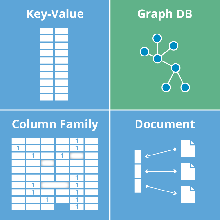
The group of NoSQL databases collectively known as aggregate stores (term coined by Martin Fowler) includes key-value stores, wide-column stores and document stores, which are all highlighted in blue below. (Next week, we’ll examine the various types of graph technologies, which are another facet of NoSQL.)

It’s worth noting that aggregate stores eschew connections between aggregates – only graph databases fully capitalize on data relationships.



In the following sections we’ll explore each of these three blue quadrants, highlighting the characteristics of each NoSQL data model, operational aspects and the main drivers for adoption.

Key-Value Stores

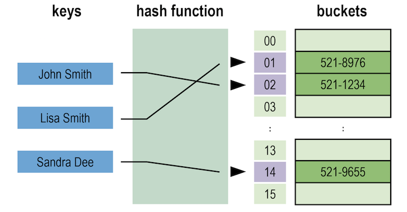
Key-value stores are large, distributed hashmap data structures that store and retrieve values organized by identifiers known as keys.

Here’s a diagram of an example key-value store.

A basic key-value store. Image based on: Jorge Stolfi.

As you can see, a bucket contains a specific number of values, and for fault-tolerance reasons, each bucket is replicated onto several machines. However, machines should never be exact copies of one another – not only for data replication purposes but also for better load balancing.

An application wishing to store or retrieve data in a key-value store only needs to know (or compute) the corresponding key, which can be as natural as a username, an email address, Cartesian coordinates, a Social Security number or a ZIP code. With a sensibly designed system, the chance of losing data due to a missing key is low.

In theory, key-value stores simply concern themselves with efficient storage and retrieval of data, unencumbered by its nature or usage. But this approach has its downsides: When extracting data from a stored value, applications often have to retrieve the entire value (which can be quite large) and then filter out any unwanted elements, which can be inefficient.

Although simple, the key-value model doesn’t offer much insight into data relationships. In order to retrieve sets of information across several records, you typically need to conduct external processing with an algorithm like MapReduce, often producing highly latent results.

However, key-value stores do have certain advantages: Notably, they’re optimized for high availability and scale. A great example of a popular key-value store is Redis.

Wide-Column Stores

Wide-column stores (also known as column family stores) are based on a sparsely populated table whose rows can contain arbitrary columns and where keys provide for natural indexing.

(Note: In the explanation below, we’ll use terminology from Apache Cassandra since it is one of the most popular wide-column stores).

In the diagram below, you can see the four building blocks of a wide-column database.

The four building blocks of a wide-column database.

The simplest unit of storage is the column itself consisting of a name-value pair. Any number of columns can then be combined into a super column, which gives a name to a particular set of columns. Columns are stored in rows, and when a row contains columns only, it is known as a column family, but when a row contains super columns, it is known as a super column family.

At first it might seem odd to include rows when the data is mostly organized via columns, but in fact, rows are vital since they provide a nested hashmap for columnar data. Consider the diagram below of a super column family mapping out a recording artist and his albums.

Storing data in a super column family

In a wide-column database, each row in the table represents a particular overarching entity (e.g., everything about an artist). These column families are containers for related pieces of data, such as the artist’s name and discography. Within the column families we find actual key-value data, such as album release dates and the artist’s date of birth.

Here’s the kicker: This row-oriented view can also be turned 90 degrees to arrive at a column-oriented view. Where each row gives a complete view of one entity, the column view naturally indexes particular aspects across the whole dataset.

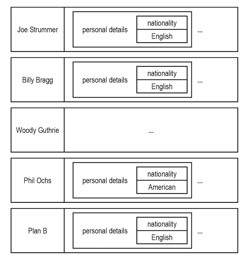
For example, let’s look at the figure below:

Keys form a natural index through rows in a wide-column database.

As you can see, by “lining up” keys we can find all the rows where the artist is English. From there it’s easy to extract complete artist data from each row. It’s not the same as the connected data as we’d find in a graph, but it does provide some insight into related entities.

Wide-column databases are distinguished from document and key-value stores not only by their more expressive data model, but also by their architecture built for distribution, scale and failover. And yet they’re still aggregate stores and as such lack JOINs.

Document Stores

Put simply, document databases store and retrieve documents just like an electronic filing cabinet. Documents can include maps and lists, allowing for natural hierarchies. In fact, document stores are most familiar to developers who are used to working with hierarchically structured documents.

At the most basic level, documents are stored and retrieved by ID. If an application remembers the IDs it’s most interested in (such as usernames), then a document store acts much like a key-value store (see above).

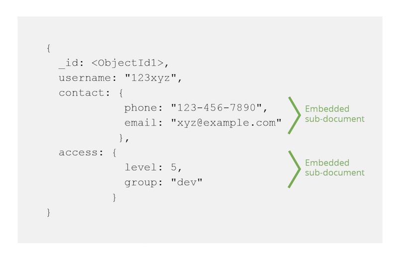
The document data model usually involves having a hierarchical JSON document as the primary data structure, and any field inside of the hierarchy can then be indexed. For example, in the diagram below the embedded sub-documents are part of the larger user document.

Embedded data in a document store. Image based on: MongoDB Data Model Design documentation.

Because document stores have a data model around disconnected entities, their major advantage is horizontal scaling. However, most document databases require developers to explicitly plan for sharding of data across instances to support this horizontal scale while key-value stores and column family stores don’t require this extra step.

To see an example of how MongoDB – one of the most popular document stores – works alongside Neo4j, check out our developer guides on polyglot persistence.

Query vs. Processing in NoSQL Aggregate Stores

On balance, the similarities between NoSQL aggregate stores are greater than the differences. While each has a different storage strategy, they all share similar characteristics when it comes to querying data.

For simple queries, aggregate stores use indexing, basic document linking or a query language.

However, for more complex queries, aggregate stores cannot generate deeper insights simply by examining individual data points. To compensate, an application typically has to identify and extract a subset of data and run it through an external processing infrastructure such as the MapReduce framework (often in the form of Apache Hadoop).

MapReduce is a parallel programming model that splits data and operates on it in parallel before gathering it back together and aggregating it to provide focused information.

For example, if we wanted to use MapReduce to count the number of Americans there are in a recording artists database, we’d need to extract all artist data and discard the non-American ones in the map phase. Then, we’d count the remaining records in the reduce phase.

But even with a lot of machines and a fast network infrastructure, MapReduce can be quite latent. So latent in fact, that often a development team needs to introduce new indexes or ad hoc queries in order to focus (and trim) the dataset for better MapReduce speeds.

Conclusion

Aggregate stores are good at storing big sets of discrete data, but they do that by sacrificing a data model, language and functionality for handling data relationships.

The spectrum of databases for discrete versus connected data.

If you try to use aggregate stores for interrelated data, it results in a disjointed development experience since you have to add a lot of code to fill in where the underlying aggregate store leaves off. And as the number of hops (or “degrees”) of the query increase, aggregate stores slow down significantly.

Graph database technology, on the other hand, embraces relationships in order to solve problems that involve context and connectedness. Consequently, they have very different design principles and a different architectural foundation.

Do aggregate stores have their perfect use cases? Certainly. But they aren’t for dealing with problems that require an understanding of how things are connected.





Catch up with the rest of the Graph Databases for Beginners series:

• Why Graph Technology Is the Future
• Why Connected Data Matters
• The Basics of Data Modeling
• Data Modeling Pitfalls to Avoid
• Why a Database Query Language Matters (More Than You Think)
• Imperative vs. Declarative Query Languages: What’s the Difference?
• Graph Theory & Predictive Modeling
• Graph Search Algorithm Basics
• Why We Need NoSQL Databases
• ACID vs. BASE Explained
• Other Graph Data Technologies
• Native vs. Non-Native Graph Technology