Under the Covers With LightRAG: Extraction and Retrieval

Solutions Engineer, Neo4j
30 min read

Remember the days when naive retrieval-augmented generation (RAG) felt like magic? Upload a few documents to a vector store, hook it up to an LLM, and voilà! Instant answers! Fast-forward to today, that naive RAG setup is the new “Hello, World!” for the new world. The bar? It’s been raised — repeatedly. There are now an estimated 30+ RAG techniques floating around (thanks to the awesome RAG_Techniques repo from NirDiamant), all chasing the same holy grail: more accuracy, reliability, and richly context-aware answers. And most importantly, with the least amount of work.
In this blog, I’ll break down yet another promising new RAG technique that has been gaining traction lately: LightRAG. It leans into the power of relationships and graphs to push the boundaries of what modern RAG systems can do.
TL;DR

- Better answers for different question types: The dual-level keyword extraction and hybrid retrieval architecture handles specific, entity-focused questions and broader, conceptual inquiries. This means users get good answers whether they ask about detailed facts or big-picture concepts.
- Smarter focus on what matters: Entities and relationships are ranked based on node and edge degree, retrieving information of the highest structural significance. This ensures that responses are not only semantically relevant but also anchored in what matters most within the knowledge graph.
- Easy to update with new information: Powered by a schema-flexible knowledge graph, new entities, facts, and relationships can be easily added. This reduces the need for retraining and re-indexing, making it ideal for organizations with frequent or evolving data.
Introduction

So what’s LightRAG? It shares similar architectural DNA with frameworks like GraphRAG, leveraging knowledge graphs (e.g., Neo4j) to enrich retrieval with structured, contextual information. But where many approaches treat graphs as an optional add-on, LightRAG makes them central to the retrieval process. Traditional RAG pipelines often rely too much on vector similarity and flat chunks. This has been proven to be great for shallow lookups, but not for answering questions that depend on understanding how things connect. Real-world data is relational by nature, and that’s where graphs shine.
Extraction Pipeline
At its core, LightRAG builds upon the idea that structured knowledge (entities and relationships) extracted from raw documents can enhance retrieval quality but without requiring a community summarization layer like Microsoft’s version of GraphRAG. The later is a technique also known as query focused summarization where given a user question and a community level, the community summaries are retrieved and given to the LLM as an enrichment step. You can read more about the different techniques on graphrag.com.

LightRAG’s pipeline takes a more streamlined path. It begins by cleaning and chunking raw documents, then uses LLMs to extract structured knowledge in the form of entities, relationships, and keywords. This extracted structure is saved into a knowledge graph and indexed into vector databases for fast semantic search in a parallel fashion. The extraction process is similar to that of GraphRAG but with some proposed enhancements which will be covered below.
Where query focused summarization leverages the power of community summaries to handle ‘global’ questions, LightRAG’s capabilities lie in how it aligns vector search and graph queries at retrieval time to provide grounded, explainable answers.
The key insight here is that LightRAG builds a multi-layered retrieval surface:
- Semantic chunks for vector search
- Graph entities and relationships for reasoning and relevance tracking
- Metadata-enriched relationships for deeper filtering or traversal
The original relationships between concepts are preserved, and entity- and relationship-level embeddings are used for retrieval in conjunction with chunk-level vector embeddings. This layered retrieval strategy provides traceability and a richer context to the LLM, enabling a more accurate and grounded response.
At a high level, LightRAG processes documents in the following way.
Document Preparation Phase
This stage handles raw document ingestion, cleaning, de-duplication, and metadata preparation.
Document Ingestion and Text Cleaning
- Remove null bytes
- Strip whitespace
The clean_text function removes null bytes and leading/trailing whitespace from the text, ensuring that it’s ready for processing.
# lightrag/utils.py
def clean_text(text: str) -> str:
    """Clean text by removing null bytes (0x00) and whitespace

    Args:
        text: Input text to clean

    Returns:
        Cleaned text
    """
    return text.strip().replace("\x00", "")
De-Duplication
- Check for duplicate content
- Remove duplicates
- Reconstruct unique content
The extracted contents are iterated to uniquely identify and prevent any content from duplication. The contents dictionary is then reconstructed to include only unique entries.
# lightrag/lightrag.py
unique_contents = {}
for id_, content_data in contents.items():
    content = content_data["content"]
    file_path = content_data["file_path"]
    if content not in unique_contents:
        unique_contents[content] = (id_, file_path)

contents = {
    id_: {"content": content, "file_path": file_path}
    for content, (id_, file_path) in unique_contents.items()
}
Content Summarization, Filtering, and Metadata Preparation
- Generate content summary
- Truncate if it exceeds max length
The get_content_summary function simply truncates the content to a specified maximum length, appending an ellipsis if the text exceeds that limit. The function effectively creates a brief excerpt, but labeling it as a “summary” might be misleading.
In my opinion, this snippet serves other practical purposes, such as quick previews and more efficient storage when handling large volumes of documents.
# lightrag/utils.py
def get_content_summary(content: str, max_length: int = 250) -> str:
    """Get summary of document content

    Args:
        content: Original document content
        max_length: Maximum length of summary

    Returns:
        Truncated content with ellipsis if needed
    """
    content = content.strip()
    if len(content) <= max_length:
        return content
return content[:max_length] + "..."- Prepare document metadata
- Filter already ingested
- Upsert document status/metadata
Each document gets enriched with metadata that includes the earlier truncated preview of the content, along with timestamps for auditability and the original file path for traceability.
# lightrag/lightrag.py
# 3. Generate document initial status
new_docs: dict[str, Any] = {
    id_: {
        "status": DocStatus.PENDING,
        "content": content_data["content"],
        "content_summary": get_content_summary(content_data["content"]),
        "content_length": len(content_data["content"]),
        "created_at": datetime.now().isoformat(),
        "updated_at": datetime.now().isoformat(),
        "file_path": content_data[
            "file_path"
        ],  # Store file path in document status
    }
    for id_, content_data in contents.items()
}

# 4. Filter out already processed documents
# Get docs ids
all_new_doc_ids = set(new_docs.keys())
# Exclude IDs of documents that are already in progress
unique_new_doc_ids = await self.doc_status.filter_keys(all_new_doc_ids)
A database lookup is performed using the MD5 hash-based document ID to verify the uniqueness of the document.
# for entities
compute_mdhash_id(dp["entity_name"], prefix="ent-")

# for relationships
compute_mdhash_id(dp["src_id"] + dp["tgt_id"], prefix="rel-")
If it does, the filter_keys function will remove it from further processing. Below is a sample input for new docs. Let’s assume that if doc-a1b2c3 has already been processed and exists in the database, the pipeline will exclude it from further processing, and the metadata records for each document are then ingested into the key-value store.
# From
new_docs = {
    "doc-a1b2c3": {
        "status": "PENDING",
        "content_summary": "Sample content 1",
        "content_length": 29,
        "file_path": "file1.txt",
        ...
    },
    "doc-123abc": {
        "status": "PENDING",
        "content_summary": "Sample content 2",
        "content_length": 24,
        "file_path": "file2.txt",
        ...
    }
}

# To
new_docs = {
    "doc-123abc": {
        "status": "PENDING",
        "content_summary": "Sample content 2",
        "content_length": 24,
        "file_path": "file2.txt",
        ...
    }
}
Semantic Enrichment Phase
The following stage focuses on converting cleaned text into usable semantic and graph structures. Once documents are cleaned, de-duplicated, and filtered in the earlier phase, LightRAG moves into its second pre-processing phase, where the real transformation begins. Here, we take unstructured text and chunk, embed, extract, and structure it into vectors and a graph. This is the bedrock of semantic search and graph-powered reasoning.
Chunking and Embedding
Chunking By Token Size
The overlap chunking strategy is used to retain semantic context across overlapping windows. There is an overlap token size of 128 by default. We won’t debate the “perfect” chunk size here — that’s a nuanced topic for another post — but the chunking function is entirely configurable via LightRAG.chunking_func.
# lightrag/operate.py
def chunking_by_token_size(
    content: str,
    split_by_character: str | None = None,
    overlap_token_size: int = 128,
    max_token_size: int = 1024,
    ...
) -> list[dict[str, Any]]:
Generate Embeddings
Once the content is chunked, each chunk is passed through your configured embedding function, which could use OpenAI, Claude, or a local embedding model.
The embedding results are stored along with metadata like full_doc_id, file_path, and content into a vector index or database, enabling traceable and explainable semantic search.
# lightrag/lightrag.py
self.chunks_vdb: BaseVectorStorage = self.vector_db_storage_cls(  # type: ignore
    namespace=make_namespace(
        self.namespace_prefix, NameSpace.VECTOR_STORE_CHUNKS
    ),
    embedding_func=self.embedding_func,
    meta_fields={"full_doc_id", "content", "file_path"},
)

chunks_vdb_task = asyncio.create_task(
    self.chunks_vdb.upsert(chunks)
)
Entity and Relationship Extraction
- Process chunks for extraction
- LLM extraction prompt
Before we can extract entities and relationships from the chunks of text, LightRAG prepares a highly structured prompt for the LLM. The structured prompt is composed using configurable entity types and few-shot examples, which enables the user with more control.
The following entity types are configured to be extracted by default. The defaults can be overridden by passing in custom entity types to tailor the extraction process to your domain.
# lightrag/prompt.py
PROMPTS["DEFAULT_ENTITY_TYPES"] = ["organization", "person", "geo", "event", "category"]

# lightrag/operate.py
entity_types = global_config["addon_params"].get(
    "entity_types", PROMPTS["DEFAULT_ENTITY_TYPES"]
)
If few-shot examples are not explicitly provided, it will default to using a set of predefined few shot examples in the prompt template located in:
# lightrag/prompt.py
PROMPTS["entity_extraction_examples"]
Each example follows the same format that we expect the LLM to return.
Sample text:
while Alex clenched his jaw, the buzz of frustration dull against the backdrop of Taylor's authoritarian certainty. It was this competitive undercurrent that kept him alert, the sense that his and Jordan's shared commitment to discovery was an unspoken rebellion against Cruz's narrowing vision of control and order.

Then Taylor did something unexpected. They paused beside Jordan and, for a moment, observed the device with something akin to reverence. "If this tech can be understood..." Taylor said, their voice quieter, "It could change the game for us. For all of us."

The underlying dismissal earlier seemed to falter, replaced by a glimpse of reluctant respect for the gravity of what lay in their hands. Jordan looked up, and for a fleeting heartbeat, their eyes locked with Taylor's, a wordless clash of wills softening into an uneasy truce.

It was a small transformation, barely perceptible, but one that Alex noted with an inward nod. They had all been brought here by different paths
Sample output:
# lightrag/prompt.py
("entity"{tuple_delimiter}"Alex"{tuple_delimiter}"person"{tuple_delimiter}"Alex is a character...")
("relationship"{tuple_delimiter}"Alex"{tuple_delimiter}"Taylor"{tuple_delimiter}"Power dynamic..."{tuple_delimiter}"conflict"{tuple_delimiter}7)
("content_keywords"{tuple_delimiter}"discovery, control, rebellion")
The prompt uses placeholder delimiters (like "{tuple_delimiter}") which are dynamically injected with defaults like:
# lightrag/prompt.py
PROMPTS["DEFAULT_TUPLE_DELIMITER"] = "<|>"
PROMPTS["DEFAULT_RECORD_DELIMITER"] = "##"
PROMPTS["DEFAULT_COMPLETION_DELIMITER"] = "<|COMPLETE|>"
A full extraction is formed by combining the elements detailed above.
# lightrag/prompt.py
PROMPTS["entity_extraction"] = """---Goal---
Given a text document that is potentially relevant to this activity and a list of entity types, identify all entities of those types from the text and all relationships among the identified entities.
Use {language} as output language.

---Steps---
1. Identify all entities. For each identified entity, extract the following information:
- entity_name: Name of the entity, use same language as input text. If English, capitalized the name.
- entity_type: One of the following types: [{entity_types}]
- entity_description: Comprehensive description of the entity's attributes and activities
Format each entity as ("entity"{tuple_delimiter}<entity_name>{tuple_delimiter}<entity_type>{tuple_delimiter}<entity_description>)

2. From the entities identified in step 1, identify all pairs of (source_entity, target_entity) that are *clearly related* to each other.
For each pair of related entities, extract the following information:
- source_entity: name of the source entity, as identified in step 1
- target_entity: name of the target entity, as identified in step 1
- relationship_description: explanation as to why you think the source entity and the target entity are related to each other
- relationship_strength: a numeric score indicating strength of the relationship between the source entity and target entity
- relationship_keywords: one or more high-level key words that summarize the overarching nature of the relationship, focusing on concepts or themes rather than specific details
Format each relationship as ("relationship"{tuple_delimiter}<source_entity>{tuple_delimiter}<target_entity>{tuple_delimiter}<relationship_description>{tuple_delimiter}<relationship_keywords>{tuple_delimiter}<relationship_strength>)

3. Identify high-level key words that summarize the main concepts, themes, or topics of the entire text. These should capture the overarching ideas present in the document.
Format the content-level key words as ("content_keywords"{tuple_delimiter}<high_level_keywords>)

4. Return output in {language} as a single list of all the entities and relationships identified in steps 1 and 2. Use **{record_delimiter}** as the list delimiter.

5. When finished, output {completion_delimiter}

######################
---Examples---
######################
{examples}

#############################
---Real Data---
######################
Entity_types: [{entity_types}]
Text:
{input_text}
######################
Output:"""
Parse Extraction Results
The raw final_result string from the LLM is further processed and returns two dictionaries:
maybe_nodes: entity name → list of entity dictsmaybe_edges: (source, target) → list of relationship dicts
# lightrag/operate.py
maybe_nodes, maybe_edges = await _process_extraction_result(
    final_result, chunk_key, file_path
)
final_result is subjected to further transformation in subsequent steps. Using the delimiters defined, LightRAG splits the full result into individual records. But what’s probably more interesting is, unlike traditional entity and relationship extraction, LightRAG goes a step further in quantifying each relationship and characterizing them semantically.
Specifically, each extracted relationship includes:
- relationship_strength — A numeric score indicating how strong or important the relationship is between the source and target entities. This allows us to model not just that two things are related, but how tightly, how frequently, or how significantly they co-occur or interact.
It’s worth noting that this relationship_strength score comes from the LLM’s interpretation, not hard data. It’s like asking someone “How close do you think these two people are?” rather than counting actual interactions. The LLM is making an educated guess based on context.
- relationship_keyword — One or more high-level keywords that summarize the nature of the relationship, capturing themes or concepts (e.g., “conflict”, “collaboration”, “influence”). These act as compact semantic tags that can be used for filtering, clustering, or graph visualization.
Together, these enrich the knowledge graph with contextual metadata that goes beyond just “Entity A is related to Entity B.” During retrieval, you can prioritize relationships based on weight (e.g., “only show me strong connections”), or discard noisy edges with low scores. The result is smarter graph traversal, more focused retrieval, and a better foundation for downstream reasoning.
Additionally, the central themes or topics present in the chunk are summarized as content_keywords. These reflect what the text is about overall and is not tied to any specific entity or relationship.
# Before
("entity"<|>"Alex"<|>"person"<|>"Alex is a character...")##
("relationship"<|>"Alex"<|>"Taylor"<|>"Power dynamic..."<|>"conflict"<|>"7")##
("content_keywords"<|>"discovery, control, rebellion")<|COMPLETE|>

# In Between
[
  '("entity"<|>"Alex"<|>"person"<|>"Alex is a character...")',
  '("relationship"<|>"Alex"<|>"Taylor"<|>"Power dynamic..."<|>"conflict"<|>"7")',
  '("content_keywords"<|>"discovery, control, rebellion")'
]

# After (Above: Entities, Below: Relationships)
["entity", "Alex", "person", "Alex is a character..."]

["relationship", "Alex", "Taylor", "Power dynamic...", "conflict", "7"]- Transform entities
- Transform relationships
The processed records will be subjected to separate transformation based on whether it’s an entity or relationship. The records will then have metadata information attached to them.
# maybe_nodes
{
  "entity_name": "Alex",
  "entity_type": "person",
  "description": "Alex is a character...",
  "source_id": "chunk-123",
  "file_path": "file1.txt"
}

# maybe_edges
{
  "src_id": "Alex",
  "tgt_id": "Taylor",
  "description": "Power dynamic...",
  "keywords": "conflict",
  "weight": 7.0,
  "source_id": "chunk-345",
  "file_path": "file1.txt"
}
Gleaning Loop (Optional Retry for Low-Confidence Chunks)
- Gleaning and retry extraction
- Merge new entities and relationships
- Check extraction loop
- Combine all results
There might be cases where the LLM misses entities or relationships in its first pass, especially in dense text chunks. LightRAG includes a simple retry mechanism called gleaning, where it prompts the LLM again (up to a configurable limit) to extract anything that might have been previously overlooked. If new entities or relationships are found, they’ll be appended to the overall results. Notice that the prompt used in the gleaning phase is more aggressive and assertive than the previous extraction prompt in order to force it to cover all ground.
# lightrag/prompt.py
PROMPTS["entity_continue_extraction"] = """
MANY entities and relationships were missed in the last extraction.

---Remember Steps---

1. Identify all entities. For each identified entity, extract the following information:
- entity_name: Name of the entity, use same language as input text. If English, capitalized the name.
- entity_type: One of the following types: [{entity_types}]
- entity_description: Comprehensive description of the entity's attributes and activities
Format each entity as ("entity"{tuple_delimiter}<entity_name>{tuple_delimiter}<entity_type>{tuple_delimiter}<entity_description>

2. From the entities identified in step 1, identify all pairs of (source_entity, target_entity) that are *clearly related* to each other.
For each pair of related entities, extract the following information:
- source_entity: name of the source entity, as identified in step 1
- target_entity: name of the target entity, as identified in step 1
- relationship_description: explanation as to why you think the source entity and the target entity are related to each other
- relationship_strength: a numeric score indicating strength of the relationship between the source entity and target entity
- relationship_keywords: one or more high-level key words that summarize the overarching nature of the relationship, focusing on concepts or themes rather than specific details
Format each relationship as ("relationship"{tuple_delimiter}<source_entity>{tuple_delimiter}<target_entity>{tuple_delimiter}<relationship_description>{tuple_delimiter}<relationship_keywords>{tuple_delimiter}<relationship_strength>)

3. Identify high-level key words that summarize the main concepts, themes, or topics of the entire text. These should capture the overarching ideas present in the document.
Format the content-level key words as ("content_keywords"{tuple_delimiter}<high_level_keywords>)

4. Return output in {language} as a single list of all the entities and relationships identified in steps 1 and 2. Use **{record_delimiter}** as the list delimiter.

5. When finished, output {completion_delimiter}

---Output---

Add them below using the same format:\n
""".strip()
Final Merge, De-Duplication
- Merge and summarize entities
- Merge and summarize relationships
After the gleaning phase, LightRAG shifts gear into aggregation mode. This is where it combines the pieces, cleans them up, and saves them into the knowledge graph and the vector database.
All occurrences of the same entities are combined and grouped across chunks. For example, if “Alex” appears in three different chunks with different descriptions, all three entries will now be grouped under all_nodes["Alex"].
Relationships are consolidated across chunks to give a consistent, canonical key regardless of the order they were extracted. This essentially treats relationships as bidirectional.
# lightrag/operate.py
for edge_key, edges in maybe_edges.items():
    sorted_edge_key = tuple(sorted(edge_key))
    all_edges[sorted_edge_key].extend(edges)
It makes sure that similar edges are treated as the same relationship.
# From
("Alex", "Taylor")
("Taylor", "Alex")

# To
sorted(("Alex", "Taylor")) → ("Alex", "Taylor")
sorted(("Taylor", "Alex")) → ("Alex", "Taylor")
Ingestion to Knowledge Graph and Vector Database
Once all chunk-level entity and relationship extractions are complete, LightRAG proceeds to merge, de-duplicate, and upsert this information into the knowledge graph and vector database. Here’s how that process unfolds.
Processing Nodes (Entities)
Each entity is retrieved using the entity_name attribute from the knowledge graph. If a matching node already exists, its existing metadata is retrieved.
- Picking the dominant
entity_type
The entity_type with the highest frequency count is picked using a frequency counter (e.g., “person” has the highest frequency of occurrence here).
# example
entity_types = ["person", "character", "person", "persona", "person", "protagonist", "character"]

# lightrag/operate.py
entity_type = sorted(
    Counter(
        [dp["entity_type"] for dp in nodes_data] + already_entity_types
    ).items(),
    key=lambda x: x[1],
    reverse=True,
)[0][0]

# result
entity_type = "person"- Combining description
Description values are combined using ||| as a separator to preserve context, if the number of fragments merged exceeds the default threshold of 6, an LLM is used to summarize them into one concise description.
merged_description = (
  "A highly observant character involved in power dynamics.|||Alex is a character..."
)
This balances completeness with readability — avoiding bloat in the knowledge graph.
- Combining
source_idandfile_path
source_id and file_path are combined; these fields aren’t summarized because they’re used for traceability and provenance.
source_id = "chunk-123|||chunk-456"
file_path = "file1.txt|||file2.txt"
Processing Relationships
Relationships are processed similarly where each edge (src_id, tgt_id) pair is looked up in the graph. If a matching relationship already exists, its existing metadata is retrieved.
- Combining descriptions and keywords
Descriptions and keywords from all edge mentions are concatenated. Similarly, if the number of fragments merged exceeds the threshold defined, an LLM is used to summarize them into one concise description.
{
  "description": "Power dynamic...|||Mentorship dynamic between Taylor and Alex.",
  "keywords": "conflict, guidance, imbalance"
}- Aggregating weight
Each relationship has a weight, representing how strong or confidently it was extracted. When the same relationship appears multiple times, weights are added up.
weight = 7.0 + 5.0 = 12.0- Combining
source_idandfile_path
Again, all source_id and file_path values are preserved for full traceability.
Upserting Nodes/Relationships Into the Knowledge Graph
LightRAG supports Neo4j as a graph store and uses Cypher queries to insert or update entities and relationships. This makes the graph queryable and explainable.
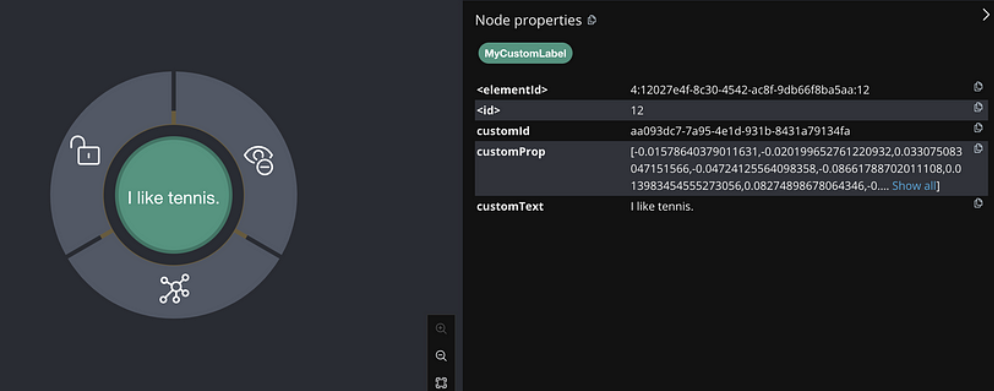
By default, LightRAG uses a generic base label for all nodes. All extracted attributes (like entity_type, description, etc.) are stored as key-value properties on that node.
// Upsert of nodes
MERGE (n:base {entity_id: $entity_id})
SET n += $properties
SET n:`%s`
In my opinion, this approach makes it easier to search and index. However, semantic clarity could be improved by using
entity_typeas the label instead of just base (e.g.,:Person,:Technology, or:Organizationmakes the graph easier to query contextually in Cypher).
// Upsert of relationships
MATCH (source:base {entity_id: $source_entity_id})
WITH source
MATCH (target:base {entity_id: $target_entity_id})
MERGE (source)-[r:DIRECTED]-(target)
SET r += $properties
RETURN r, source, target
Upserting Into Vector Database
To enable semantic search, LightRAG also embeds each entity and relationship into a vector and stores it in a vector database.
For each entity and relationship, it builds a content string:
# For entities
content = f"{entity_name}\n{description}"
# e.g., "Alex\nAlex is a character..."

# For relationship
content = f"{src_id}\t{tgt_id}\n{keywords}\n{description}"
# e.g., "Alex\tTaylor\nconflict, guidance\nPower dynamic between them"
This content field is what gets embedded into a high-dimensional vector via an embedding model.
Each of these is stored in a separate vector document.
# entities
{
  "_id": "ent-8b14c7...",
  "entity_name": "Alex",
  "entity_type": "person",
  "content": "Alex\nAlex is a character who is highly observant of power dynamics.",
  "source_id": "chunk-123|||chunk-456",
  "file_path": "file1.txt|||file2.txt",
  "vector": [0.015, -0.782, 0.431, ...]
}

# relationships
{
  "_id": "rel-7f91de...",
  "src_id": "Alex",
  "tgt_id": "Taylor",
  "keywords": "conflict, guidance",
  "content": "...",
  "source_id": "chunk-345|||chunk-567",
  "file_path": "file1.txt|||file2.txt",
  "vector": [0.73, -0.46, 0.2, ...]
}
By persisting knowledge in both a graph database and a vector database, LightRAG unlocks a powerful hybrid retrieval model similar to GraphRAG, which we will discuss more in detail below.
Neo4j offers the capabilities of both a knowledge graph and a vector database, enabling hybrid retrieval within a single platform.
Retrieval Process: A Dual-Level Hybrid Strategy

The retrieval strategy used in LightRAG combines graph traversal with semantic vector similarity. This hybrid approach aims to be accurate and explainable, which is ideal for tasks that require contextual depth and traceability. For this discussion, we’ll focus on the hybrid retrieval strategy.
Overview: Two Parallel Retrieval Paths
In LightRAG’s mix mode, retrieval happens along two parallel paths:
(A) get_kg_context() retrieves structured knowledge from the graph and surrounding documents using:
- Dual-level keyword semantic search
- Graph traversal over entities and relationships
(B) get_vector_context() retrieves unstructured semantic matches using:
- Full query embedding (with optional chat history)
- Pure vector similarity search across raw document chunks
# lightrag/operate.py
kg_context, vector_context = await asyncio.gather(
    get_kg_context(), get_vector_context()
)
Dual-Level Keyword Extraction
One of the most interesting aspects of this process is how LightRAG handles a user’s query using a concept the authors call dual-level keyword extraction. In this approach, an LLM is prompted to extract two complementary sets of keywords — high-level and low-level keywords — as shown in the prompt below:
# lightrag/prompts.py
PROMPTS["keywords_extraction"] = """---Role---

You are a helpful assistant tasked with identifying both high-level and low-level keywords in the user's query and conversation history.

---Goal---

Given the query and conversation history, list both high-level and low-level keywords. High-level keywords focus on overarching concepts or themes, while low-level keywords focus on specific entities, details, or concrete terms.

---Instructions---

- Consider both the current query and relevant conversation history when extracting keywords
- Output the keywords in JSON format, it will be parsed by a JSON parser, do not add any extra content in output
- The JSON should have two keys:
  - "high_level_keywords" for overarching concepts or themes
  - "low_level_keywords" for specific entities or details

######################
---Examples---
######################
{examples}

#############################
---Real Data---
######################
Conversation History:
{history}

Current Query: {query}
######################
The `Output` should be human text, not unicode characters. Keep the same language as `Query`.
Output:

"""- High-level keywords: broad concepts or themes
- Low-level keywords: specific entities or terms
Let’s say the user query is:
“What are the environmental consequences of deforestation on biodiversity?”
{
  "high_level_keywords": ["Environmental consequences", "Deforestation", "Biodiversity loss"],
  "low_level_keywords": ["Species extinction", "Habitat destruction", "Carbon emissions", "Rainforest", "Ecosystem"]
}
High-level keywords help LightRAG understand what the query is about. Low-level keywords help LightRAG identify who or what it’s about. Together, they drive a hybrid retrieval strategy that’s both explainable and semantically rich.
(A) Dual-Level Keyword Retrieval
LightRAG takes a hybrid approach that blends semantic vector search with the power of graphs to power a grounded, explainable and flexible retrieval. Both paths leverage 1) vector similarity to surface semantically relevant content and 2) enrich it with graph traversal and metadata. For context, the discussion below is based on Neo4j’s implementation.

1) High-Level Keywords — Relationship-Centric Context Retrieval
Recall that in the dual-level extraction process, each relationship is summarized using high-level keywords. From the extraction prompt, the keywords refer to abstract terms that encapsulate the overarching nature of the connection, rather than its surface details.
Step 1: Vector Similarity Search
These embedded content strings were previously indexed in a vector store during the extraction pipeline earlier.
# For relationship
content = f"{src_id}\t{tgt_id}\n{keywords}\n{description}"
The high-level keywords extracted from the user’s query are then converted into a query embedding, which is then used for vector similarity comparison against the former to find semantically relevant relationships, even if the exact keywords don’t appear.
#lightrag/operate.py
results = await relationships_vdb.query(
    keywords, top_k=query_param.top_k, ids=query_param.ids
)
Step 2: Retrieving Relationship/Edge Properties From the Knowledge Graph
With the vector similarity search results, we’ll use the node pairs (src_id and tgt_id) to subsequently query the knowledge graph for an actual edge between the two matched nodes. This returns all edge properties — weight , description , keywords , source_id.
#lightrag/kg/neo4j_impl.py
query = """
    MATCH (start:base {entity_id: $source_entity_id})-[r]-(end:base {entity_id: $target_entity_id})
    RETURN properties(r) as edge_properties
"""
Step 3a: Quantifying Graph Importance of the Relationship
Retrieves the degree of each source node and target node pair involved in the relationship. Computes the sum of their degrees to represent the combined centrality of the edge.
#lightrag/kg/neo4j_impl.py
query = """
    MATCH (n:base {entity_id: $entity_id})
    OPTIONAL MATCH (n)-[r]-()
    RETURN COUNT(r) AS degree
"""
Step 3b: Sort Relationships by Rank and Weight
The enriched relationships are sorted in descending order using two keys:
- rank — How central the nodes are (sum of degrees)
- weight — How strong the relationship is (from earlier extraction)
This ensures that well-connected and highly relevant relationships are surfaced first.
#lightrag/operate.py
edge_datas = sorted(
    edge_datas, key=lambda x: (x["rank"], x["weight"]), reverse=True
)
This process aims to ensure answers generated are not just relevant but highly centralized within the graph.
Step 3c: Retrieve Node Properties From the Knowledge Graph
After sorting the relationships, metadata for each unique entity involved in those top-ranked edges is retrieved. This includes attributes like entity_type and description.
#lightrag/kg/neo4j_impl.py
query = "MATCH (n:base {entity_id: $entity_id}) RETURN n"

...

node = records[0]["n"]
node_dict = dict(node) # Node metadata returned
...
return node_dict
Similarly, node_degree is calculated for each entity pair for subsequent ranking. If the total token size of the assembled node_datas exceeds the limit max_token_size, the result will be truncated to limit the token size.
#lightrag/operate.py
node_datas = [
    {**n, "entity_name": k, "rank": d}
    for k, n, d in zip(entity_names, node_datas, node_degrees)
    if n is not None
]
Step 4: Retrieve Text Chunks From Key-Value Store
Using the ranked relationships from edge_datas in Step 3b), chunk IDs for each relationship’s source_id (which may look like "chunk-001|||chunk-002") are split based on the delimiter and searched in the key-value store to retrieve the full chunk metadata. The final output is then sorted based on the original order of ranked relationships and then truncated if it exceeds the max_token_size.
#lightrag/operate.py
async def fetch_chunk_data(c_id, index):
    if c_id not in all_text_units_lookup:
        chunk_data = await text_chunks_db.get_by_id(c_id)
        # Only store valid data
        if chunk_data is not None and "content" in chunk_data:
            all_text_units_lookup[c_id] = {
                "data": chunk_data,
                "order": index,
            }
Step 5: Combining Node, Relationship and Chunk Context
After retrieving:
- Semantically matched relationships via high-level keywords
- Corresponding edge metadata from the knowledge graph
- The entities involved in those edges (source and target nodes)
- The document chunks that referenced or supported those entities and relationships
The transformation assembles a prompt-ready, structured context in three sections:
#lightrag/operate.py
# structuring entities
entites_section_list.append(
    [
        i,
        n["entity_name"],
        n.get("entity_type", "UNKNOWN"),
        n.get("description", "UNKNOWN"),
        n["rank"],
        created_at,
        file_path,
    ]
)
entities_context = list_of_list_to_csv(entites_section_list)
...
# structuring relationships
relations_section_list = [
    [
        "id",
        "source",
        "target",
        "description",
        "keywords",
        "weight",
        "rank",
        "created_at",
        "file_path",
    ]
]
relations_context = list_of_list_to_csv(relations_section_list)
...
# structuring chunks
text_units_section_list = [["id", "content", "file_path"]]
text_units_context = list_of_list_to_csv(text_units_section_list)
...
return entities_context, relations_context, text_units_context
These are returned as CSV-formatted string blocks, which seems to be advantageous as highlighted by another article, making it easy for the model to parse, reason over, and generate responses from.
#lightrag/operate.py
return entities_context, relations_context, text_units_context

#sample
-----Entities-----
```csv
id,entity,type,description,...
0,Taylor,Person,Authority figure...,3,...

-----Relationships-----
```csv
id,source,target,description,keywords,weight,...
0,Alex,Taylor,Power dynamic...,conflict,7,...

-----Sources-----
```csv
id,content,file_path
0,"Alex and Taylor argued...",file1.txt
2) Low-Level Keywords — Entity-Centric Context Retrieval
Similarly, during the dual-level extraction process, each entity is summarized using low-level keywords; they are the specific nouns, terms or concepts mentioned directly in the user’s query. These low-level keywords drive entity-focused retrieval where the most semantically and structurally relevant nodes from the knowledge graph are surfaced.
Step 1: Vector Similarity Search
Each entity’s content string was embedded in the vector store during the extraction pipeline using the format below.
# For entities
content = f"{entity_name}\n{description}"
# e.g., "Alex\nAlex is a character..."
Identical to high-level relationship embeddings, these entity vectors were pre-indexed into the vector store. Low-level keywords are embedded at query time and compared against this index to retrieve semantically similar entities/nodes.
# lightrag/operate.py
results = await entities_vdb.query(
    query, top_k=query_param.top_k, ids=query_param.ids
)
Step 2: Retrieve Node Properties From the Knowledge Graph
Once vector similarity results are returned, each matched entity/node is looked up in the knowledge graph to retrieve its properties.
#lightrag/kg/neo4j_impl.py
query = "MATCH (n:base {entity_id: $entity_id}) RETURN n"

...

node = records[0]["n"]
node_dict = dict(node) # Node metadata returned
...
return node_dict
Step 3a: Quantifying Graph Importance of the Entity
Just as relationships are ranked by edge centrality, entities are ranked by node degree, which is calculated based on the number of relationships a node has.
#lightrag/kg/neo4j_impl.py
query = """
    MATCH (n:base {entity_id: $entity_id})
    OPTIONAL MATCH (n)-[r]-()
    RETURN COUNT(r) AS degree
"""
A highly connected node is more likely to be influential or serve as a bridge in multihop reasoning.
Step 3b: Sort Entities by Degree (Rank)
Each entity is assigned a rank based on its node degree. The list of entities is sorted and then truncated based on the defined token limit.
# lightrag/operate.py
node_datas = [
    {**n, "entity_name": k, "rank": d}
    for k, n, d in zip(entity_names, node_datas, node_degrees)
    if n is not None
]
Step 3c: Retrieve Related Relationships From the Knowledge Graph
To enrich entity context, one–hop relationships are gathered for each retrieved entity. For each entity name, the one-hop edges are retrieved giving a list of node pairs.
#lightrag/kg/neo4j_impl.py
query = """MATCH (n:base {entity_id: $entity_id})
        OPTIONAL MATCH (n)-[r]-(connected:base)
        WHERE connected.entity_id IS NOT NULL
        RETURN n, r, connected"""
...
source_label = (
    source_node.get("entity_id")
    if source_node.get("entity_id")
    else None
)
target_label = (
    connected_node.get("entity_id")
    if connected_node.get("entity_id")
    else None
)
if source_label and target_label:
    edges.append((source_label, target_label))
...
return edges
For each unique set of node pairs, edge/relationship metadata is fetched in parallel with the information of edge degree (sum of degrees of source and target node).
#lightrag/operate.py
all_edges_pack, all_edges_degree = await asyncio.gather(
    asyncio.gather(*[knowledge_graph_inst.get_edge(e[0], e[1]) for e in all_edges]),
    asyncio.gather(
        *[knowledge_graph_inst.edge_degree(e[0], e[1]) for e in all_edges]
    ),
)
Cypher query for the retrieval of edge properties:
#lightrag/kg/neo4j_impl.py
query = """
MATCH (start:base {entity_id: $source_entity_id})-[r]-(end:base {entity_id: $target_entity_id})
RETURN properties(r) as edge_properties
"""
After the edge metadata and edge degree scores are collected, each relationship is represented as a dictionary that includes the source and target nodes, description, computed rank, and weight. These relationships are then sorted in descending order, first by rank (i.e., degree centrality), then by weight, then added to the final context.
#lightrag/operate.py
all_edges_data = [
    {"src_tgt": k, "rank": d, **v}
    for k, v, d in zip(all_edges, all_edges_pack, all_edges_degree)
    if v is not None
]
all_edges_data = sorted(
    all_edges_data, key=lambda x: (x["rank"], x["weight"]), reverse=True
)
This sorting process is vital for the identification of highly influential relationships.
Step 4: Retrieve Text Chunks From the Key-Value Store
Similar to the relationship-based approach, this alternative implementation retrieves text chunks, but starts from ranked entity nodes rather than relationships. Both approaches follow the same core pattern:
- Extract chunk IDs from source fields
- Retrieve full chunk data from the key-value store
- Sort by relevance and truncate based on defined token limits
The key difference in this implementation is the relationship analysis. While the first approach directly retrieves chunks referenced by relationships, this version:
- Identifies one-hop neighboring entities in the knowledge graph
- Counts relationship occurrences for each chunk
- Uses these counts as an additional ranking factor
# Retrieve chunks with batch processing
    batch_size = 5
    results = []
    for i in range(0, len(tasks), batch_size):
        batch_tasks = tasks[i : i + batch_size]
        batch_results = await asyncio.gather(
            *[text_chunks_db.get_by_id(c_id) for c_id, _, _ in batch_tasks]
        )
        results.extend(batch_results)

    # Track relationship density for each chunk
    for (c_id, index, this_edges), data in zip(tasks, results):
        all_text_units_lookup[c_id] = {
            "data": data,
            "order": index,
            "relation_counts": 0,  # Relationship density tracking
        }
The final output is sorted by the original entity ranking order first, then by relationship density, ensuring that chunks that connect multiple entities are prioritized.
# Sort by entity order and relationship density
all_text_units = sorted(
    all_text_units, key=lambda x: (x["order"], -x["relation_counts"])
)

# Truncate to respect token limits
all_text_units = truncate_list_by_token_size(
    all_text_units,
    key=lambda x: x["data"]["content"],
    max_token_size=query_param.max_token_for_text_unit,
)
What’s unique in the entity-centric path is that chunk scoring incorporates graph neighbor overlap.
Step 5: Combining Node, Relationship, and Chunk Context
Regardless of whether entities or relationships served as the starting point for retrieval, both approaches are similar in the post-processing of retrieval outputs. These components are then finally transformed into a structured, prompt-ready CSV-formatted context. Refer to Step 5 in the section under Relationship-Centric Context Retrieval above for an in-depth explanation of how each component is extracted and assembled.
Combined Context — Relationship- and Entities-Centric
After separately retrieving context using both low-level (entities) and high-level (relationships) keywords, the combined contexts are again cleaned, de-duplicated, and recombined into CSV-formatted string blocks.
#lightrag/utils.py
def process_combine_contexts(hl: str, ll: str):
    header = None
    list_hl = csv_string_to_list(hl.strip())
    list_ll = csv_string_to_list(ll.strip())
...
    combined_sources = []
    seen = set()

    for item in list_hl + list_ll:
        if item and item not in seen:
            combined_sources.append(item)
            seen.add(item)
...
    for i, item in enumerate(combined_sources, start=1):
        combined_sources_result.append(f"{i},\t{item}")

    return "\n".join(combined_sources_result)
(B) Pure Semantic Vector Similarity Retrieval
While the dual-level keyword retrieval (discussed in Section A) focuses on retrieval via knowledge graph, LightRAG simultaneously runs a semantic vector search in parallel.
Step 1: Query Augmentation With Conversation History
To make the vector search more conversationally aware, the user’s current query is augmented with the conversation history.
#lightrag/operate.py
async def get_vector_context():
    # Consider conversation history in vector search
    augmented_query = query
    if history_context:
        augmented_query = f"{history_context}\n{query}"
...
The addition of conversation history aims to capture ongoing intent, topic continuity, and implicit references from earlier turns, which could be useful for multi-turn interactions.
Step 2: Retrieval Via Vector Store and Key-Value Store
The augmented query is then embedded and used to retrieve semantically similar chunks from a pre-indexed vector store. For each result, the actual content is also retrieved from a key-value store using the unique chunk ID.
#lightrag/operate.py
# Reduce top_k for vector search in hybrid mode since we have structured information from KG
mix_topk = min(10, query_param.top_k)
results = await chunks_vdb.query(
    augmented_query, top_k=mix_topk, ids=query_param.ids
)
if not results:
    return None
# key-value chunk lookup
chunks_ids = [r["id"] for r in results]
chunks = await text_chunks_db.get_by_ids(chunks_ids)
When running in hybrid mode, the vector search uses a smaller top_k value since the knowledge graph already provides structured information.
Step 3: Chunk Metadata Enrichment
Each chunk is then formatted and enriched with important metadata:
- File path
- Creation timestamp
#lightrag/operate.py
# Include time information in content
formatted_chunks = []
for c in maybe_trun_chunks:
    chunk_text = "File path: " + c["file_path"] + "\n" + c["content"]
    if c["created_at"]:
        chunk_text = f"[Created at: {time.strftime('%Y-%m-%d %H:%M:%S', time.localtime(c['created_at']))}]\n{chunk_text}"
    formatted_chunks.append(chunk_text)
...
return "\n--New Chunk--\n".join(formatted_chunks)
The chunks are carefully formatted with the --New Chunk-- delimiter to avoid context bleeding across chunks and ease of tracking based on timestamp.
Combining Hybrid Retrieval Results
After retrieving results from both the knowledge graph and document chunk vector search pathways, the two retrieval results will be carefully merged. This marks the final phase of the retrieval pipeline before the answer generation prompt is constructed.
#lightrag/prompts.py
sys_prompt = PROMPTS["mix_rag_response"].format(
    kg_context=kg_context or "No relevant knowledge graph information found",
    vector_context=vector_context or "No relevant text information found",
    response_type=query_param.response_type,
    history=history_context,
)

PROMPTS["mix_rag_response"] = '''
---Role---

You are a helpful assistant responding to user query about Data Sources provided below.

---Goal---

Generate a concise response based on Data Sources...

---Conversation History---
What did we discuss about deforestation last time?

---Data Sources---

1. From Knowledge Graph(KG):
Alex → Taylor: "Power dynamic conflict" [2023-10-15], weight: 7

2. From Document Chunks(DC):
[Created at: 2023-11-12 14:02:31]
File path: reports/biodiversity_impacts.txt
Deforestation disrupts ecosystems and can lead to extinction-level threats...

---Response Rules---
- Use markdown formatting with appropriate section headings
- Organize in sections like: **Causes**, **Consequences**, **Recent Observations**
- Reference up to 5 most important sources with `[KG/DC] file_path`
'''
This approach provides the LLM with both structured knowledge graph information and unstructured vector-retrieved content, offering complementary perspectives on the user’s query:
- Knowledge graph context: Explicit entities, relationships, and supporting facts with clear structure
- Vector context: Broader semantic matching with full textual context
By combining these approaches, LightRAG leverages the strengths of both retrieval methods:
- Knowledge graphs excel at capturing explicit relationships and structured information.
- Vector search excels at capturing semantic similarity and implicit connections.
The resulting hybrid context delivers more comprehensive, accurate, and contextually grounded responses to user queries.
Summary
The authors of LightRAG have introduced a smart step forward in how we connect language models to knowledge. By bringing together graph-based reasoning and semantic search, it offers the best of both worlds — something most systems don’t achieve.
What makes it special is how graph structure is used to prioritize information. Instead of just storing facts in a graph, it uses connection patterns to determine what’s most important. This means the system surfaces central, relevant information first rather than just finding keyword matches.
The practical benefits are clear: With its flexible design, you can add new information without rebuilding everything. This makes it particularly valuable for businesses where knowledge constantly evolves. Take LightRAG for a spin on GitHub! Leave a comment, or connect with me via email or on LinkedIn.
See you next time!
Under the Covers With LightRAG: Extraction and Retrieval was originally published in Neo4j Developer Blog on Medium, where people are continuing the conversation by highlighting and responding to this story.
The Developer’s Guide:
How to Build a Knowledge Graph
This ebook gives you a step-by-step walkthrough on building your first knowledge graph.
Share Article


Explore
Related Articles


Integrating Neo4j With LangChain4j for GraphRAG Vector Stores and Retrievers