Graph Algorithms in Neo4j: All Pairs Shortest Path

Graph algorithms provide the means to understand, model and predict complicated dynamics such as the flow of resources or information, the pathways through which contagions or network failures spread, and the influences on and resiliency of groups.

This blog series is designed to help you better utilize graph analytics and graph algorithms so you can effectively innovate and develop intelligent solutions faster using a graph database .

Last week we took our second look at pathfinding and graph search algorithms with a focus on the Single Source Shortest Path algorithm, using examples from Neo4j.



This week we will examine another of these algorithms with a look at the All Pairs Shortest Path algorithm, which is used to evaluate alternate routes for situations such as a freeway backup or network capacity. It’s also key in logical routing to offer multiple paths, for example, call routing alternatives in case of a failure.

About All Pairs Shortest Path

The All Pairs Shortest Path (APSP) algorithm calculates the shortest (weighted) path between all pairs of nodes. This algorithm has optimizations that make it quicker than calling the Single Source Shortest Path algorithm for every pair of nodes in the graph.

Some pairs of nodes might not be reachable from each other, so no shortest path exists between these pairs. In this scenario, the algorithm returns infinity value as a result between these pairs of nodes.

When Should I Use All Pairs Shortest Path?

• The All Pairs Shortest Path algorithm is used in urban service system problems, such as the location of urban facilities or the distribution or delivery of goods. One example of this is determining the traffic load expected on different segments of a transportation grid. For more information, see Urban Operations Research.
• All Pairs Shortest Path is used as part of the REWIRE data center design algorithm, which finds a network with maximum bandwidth and minimal latency. There are more details about this approach in the following academic paper: ”REWIRE: An Optimization-based Framework for Data Center Network Design.”

All Pairs Shortest Path Example

Let’s calculate All Pairs Shortest Path on a small dataset.

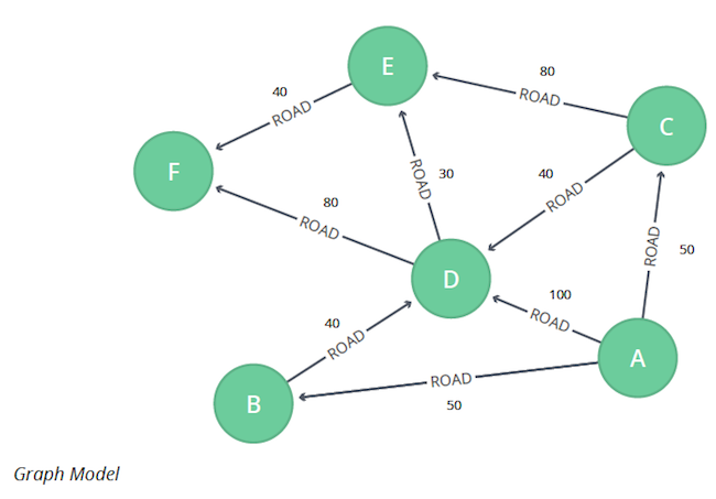
The following Cypher statement creates a sample graph containing locations and connections between them.

MERGE (a:Loc {name:"A"})
MERGE (b:Loc {name:"B"})
MERGE (c:Loc {name:"C"})
MERGE (d:Loc {name:"D"})
MERGE (e:Loc {name:"E"})
MERGE (f:Loc {name:"F"})
MERGE (a)-[:ROAD {cost:50}]->(b)
MERGE (a)-[:ROAD {cost:50}]->(c)
MERGE (a)-[:ROAD {cost:100}]->(d)
MERGE (b)-[:ROAD {cost:40}]->(d)
MERGE (c)-[:ROAD {cost:40}]->(d)
MERGE (c)-[:ROAD {cost:80}]->(e)
MERGE (d)-[:ROAD {cost:30}]->(e)
MERGE (d)-[:ROAD {cost:80}]->(f)
MERGE (e)-[:ROAD {cost:40}]->(f);

Now we run the All Pairs Shortest Path algorithm to find the shortest path between every pair of nodes. Execute the following query.

CALL algo.allShortestPaths.stream("cost",{nodeQuery:"Loc",defaultValue:1.0})
YIELD sourceNodeId, targetNodeId, distance
WITH sourceNodeId, targetNodeId, distance
WHERE algo.isFinite(distance) = true
MATCH (source:Loc) WHERE id(source) = sourceNodeId
MATCH (target:Loc) WHERE id(target) = targetNodeId
WITH source, target, distance WHERE source <> target
RETURN source.name AS source, target.name AS target, distance
ORDER BY distance DESC
LIMIT 10

This query returned the top 10 pairs of nodes that are the furthest away from each other. F and E appear to be the most distant from the others.

Conclusion

For the past few weeks we’ve covered a few use cases with our look at pathfinding and graph search algorithms, including this week’s look at All Pairs Shortest Path.

Next week we will continue our examination of these types of algorithms with an overview of the Minimum Weight Spanning Tree algorithm, which calculates the paths along a connected tree structure with the smallest value (weight of the relationship such as cost, time or capacity) associated with visiting all nodes in the tree.