3 RDBMS & Graph Database Deployment Strategies (Polyglot & More)
8 min read

Whether you’re ready to move your entire legacy RDBMS into a graph database, you’re syncing databases for polyglot persistence or you’re just conducting a brief proof of concept, at some point you’ll want to bring a graph database into your organization or architecture.
Once you’ve decided on your deployment strategy, you’ll then need to move some (or all) of your data from your relational database into a graph database. In this blog post, we’ll show you how to make that process as smooth and seamless as possible.
Your first step is to ensure you have a proper understanding of the native graph property model (i.e., nodes, relationships, labels, properties and relationship-types), particularly as it applies to your given domain.
In fact, you should at least complete a basic graph model on a whiteboard before you begin your data import. Knowing your data model ahead of time – and the deployment strategy in which you’ll use it – makes the import process significantly less painful.
In this RDBMS & Graphs blog series, we’ll explore how relational databases compare to their graph counterparts, including data models, query languages, deployment strategies and more. In previous weeks, we’ve explored why RDBMS aren’t always enough, graph basics for the RDBMS developer, relational vs. graph data modeling and SQL vs. Cypher as query languages.
This week, we’ll discuss three different database deployment strategies for relational and graph databases – as well as how to import your RDBMS data into a graph.
Three Database Deployment Strategies for Graphs and RDBMS
There are three main strategies to deploying a graph database relative to your RDBMS. Which strategy is best for your application or architecture depends on your particular goals.
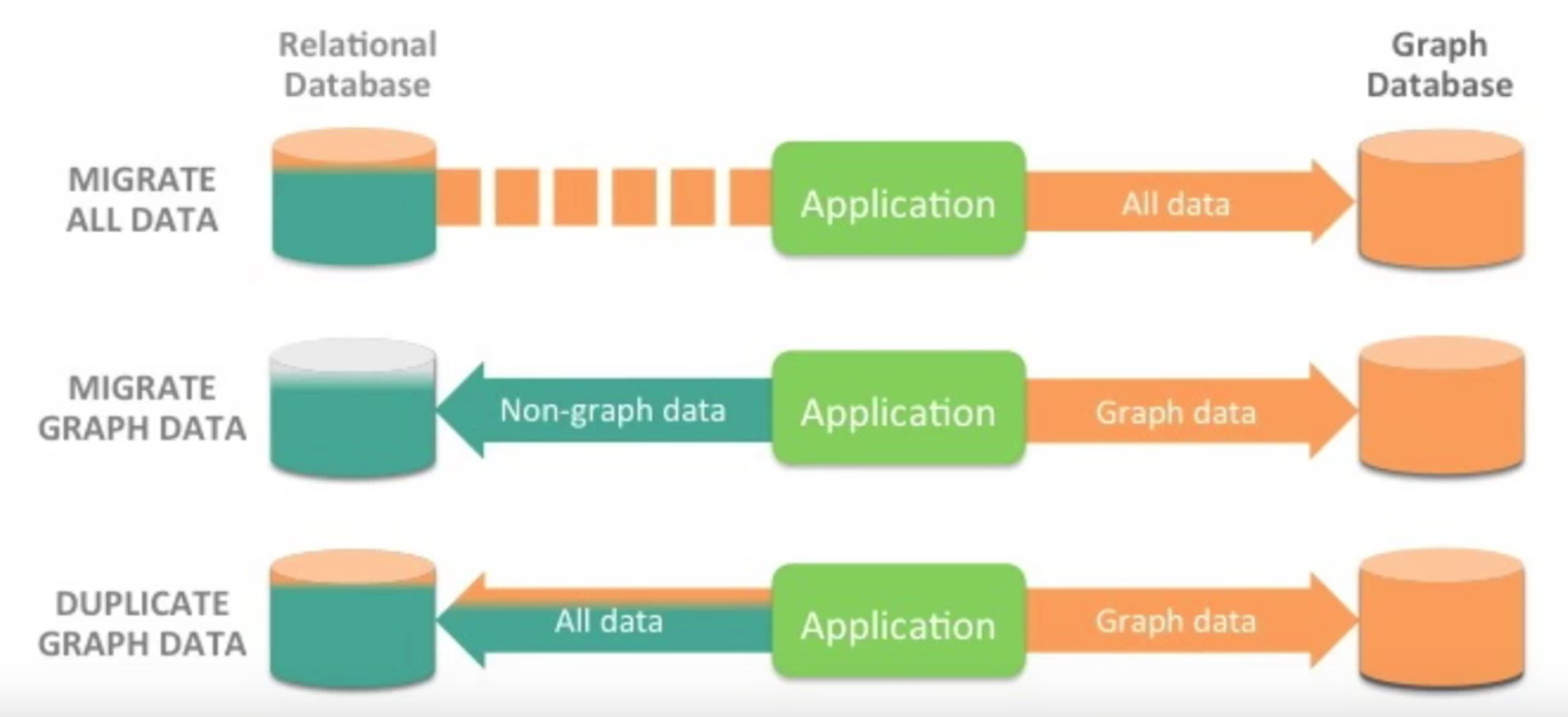
Below, you can see each of the deployment strategies for both a relational and graph database:
The three most common database deployment strategies for relational and graph databases.
First, some development teams decide to abandon their relational database all together and migrate all of their data into a graph database. This is typically a one-time, bulk migration.
Second, other developers continue to use their relational database for any use case that relies on non-graph, tabular data. Then, for any use cases that involve a lot of JOINs or data relationships, they store that data in a graph database.
Third, some development teams duplicate all of their data into both a relational database and a graph database. That way, data can be queried in whatever form is the most optimal for the queries they’re trying to run.
The second and third strategies are considered polyglot persistence, since both approaches use a data store according to its strengths. While this introduces additional complexity into an application’s architecture, it often results in getting the most optimized results from the best database for the query.
None of these is the “correct” strategy for deploying an RDBMS and a graph. Your team should consider your application goals, frequent use cases and most common queries and choose the appropriate solution for your particular environment.
Extracting Your Data from an RDBMS
No matter your given strategy, if you decide you need to import your relational data into a graph database, the first step is to extract it from your existing RDBMS.
Most all relational databases allow you to dump both whole tables or whole datasets, as well as carry results to CSV and to post queries. These tasks are usually just a copy function of the database itself. Of course, in many cases the CSV file resides on the database, so you have to download it from there, which can be a challenge.
Another option is to access your relational database with a database driver like JDBC or another driver to extract the datasets you want to pull out.
Also, if you want to set up a syncing mechanism between your relational and graph databases, then it makes sense to regularly pull the given data according to a timestamp or another updated flag so that data is synced into your graph.
Another facet to consider is that many relational databases aren’t designed or optimized for exporting large amounts of data within a short time period. So if you’re trying to migrate data directly from an RDBMS to a graph, the process might stall significantly.
For example, in one case a Neo4j customer had a large social network stored in a MySQL cluster. Exporting the data from the MySQL database took three days; importing it into Neo4j took just three hours.
One final tip before you begin: When you write to disk, be sure to disable virus scanners and check your disk schedule so you get the highest disk performance possible. It’s also worth checking any other options that might increase performance during the import process.
Importing Data via LOAD CSV
The easiest way to import data from your relational database is to create a CSV dump of individual entity-tables and JOIN-tables. The CSV format is the lowest common denominator of data formats between a variety of different applications. While the CSV format itself is unpopular, it’s also the easiest to work with when it comes to importing data into a graph database.
In Neo4j specifically, LOAD CSV is a Cypher keyword that allows you to load CSV files from HTTP or file URLs into your database. Each row of data is made available to your Cypher statement and then from those rows, you can actually create or update nodes and relationships within your graph.
The LOAD CSV command is a powerful way of converting flat data (i.e. CSV files) into connected graph data. LOAD CSV works both with single-table CSV files as well as with files that contain a fully denormalized table or a JOIN of several tables.
LOAD CSV allows you to convert, filter or de-structure import data during the import process. You can also use this command to split areas, pull out a single value or iterate over a certain list of attributes and then filter them out as attributes.
Finally, with LOAD CSV you can control the size of transactions so you don’t run into memory issues with a certain keyword, and you can run LOAD CSV via the Neo4j shell (and not just the Neo4j browser) which makes it easier it script your data imports.
In summary, you can use Cypher’s LOAD CSV command to:
- Ingest data, accessing columns by header name or offset
- Convert values from strings to different formats and structures (
toFloat,split, …) - Skip rows to be ignored
MATCHexisting nodes based on attribute lookupsCREATEorMERGEnodes and relationships with labels and attributes from the row dataSETnew labels and properties orREMOVEoutdated ones
A LOAD CSV Example
Here’s a brief example of importing a CSV file into Neo4j using the LOAD CSV Cypher command.
Example file: persons.csv
name;email;dept

"Lars Higgs";"lars@higgs.com";"IT-Department"

"Maura Wilson";"maura@wilson.com";"Procurement"
Cypher statement:
LOAD CSV FROM 'file:///data/persons.csv' WITH HEADERS AS line

FIELDTERMINATOR ";"

MERGE (person:Person {email: line.email}) ON CREATE SET p.name = line.name

MATCH (dep:Department {name:line.dept})

CREATE (person)-[:EMPLOYEE]->(dept)
You can import multiple CSV files from one or more data sources (including your RDBMS) to enrich your core domain model with other information that might add interesting insights and capabilities.
Other, dedicated import tools help you import larger volumes (10M+ rows) of data efficiently, as described below.
The Command-Line Bulk Loader
The neo4j-import command is a scalable input tool for bulk inserts. This tool takes CSV files and scales them across all of your available CPUs and disk capacity, putting the data into a stage architecture where each input step is parallelized if possible. Then, the tool stages step-by-step input using some advanced in-memory compression for creating new graph structures.
The command-line bulk loader is lightning fast, able to import up to one million records per second and handle large datasets of several billion nodes, relationships and properties. Note that because of these performance optimizations the neo4j-import tool can only be used for initial database population.
Loading Data Using Cypher
For importing data into a graph database, you can also use the Neo4j REST API to run Cypher statements yourself. With this API, you can run, create, update and merge statements using Cypher.
The transactional Cypher HTTP endpoint is available to all drivers. You can also use the HTTP endpoint directly from an HTTP client or an HTTP library in your language.
Using the HTTP endpoint (or another API), you can pull the data out of your relational database (or other data source) and convert it into parameters for Cypher statements. Then you can batch and control import transactions from there.
From Neo4j 2.2 onwards, Cypher also works really well with highly concurrent writes. In one test, one million nodes and relationships per second were inserted with highly concurrent Cypher statements using this method.
The Cypher-based loading method works with a number of different drivers, including the JDBC driver. If you have an ETL tool or Java program that already uses a JDBC tool, you can use Neo4j’s JDBC driver to import data into Neo4j because Cypher statements are just query strings (more on the JDBC driver next week). In this scenario, you can provide parameters to your Cypher statements as well.
Other RDBMS-to-Graph Import Resources:
This blog post has only covered the three most common methods for importing (or syncing) data in a graph database from a relational store.
The following are further resources on additional methods for data import, as well as more in-depth guides on the three methods discussed above:
- Guide: Data Import
- Manual: LOAD CSV
- Webinar: Data Import
- Guide: CSV Import
- Tool: Direct RDBMS Import
- Tool: SQL to Neo4j Import
- Blog: Importing AdventureWorks Data into Neo4j
- Web-based CSV import app
- Neo4j for Relational MetaData (SQLServer)
Next week we’ll take a look at connecting to a graph database via drivers and other integrations.
Want to learn more on how relational databases compare to their graph counterparts? Download this ebook, The Definitive Guide to Graph Databases for the RDBMS Developer, and discover when and how to use graphs in conjunction with your relational database.
Catch up with the rest of the RDBMS & Graphs series:


