Reloading my Beergraph - using an in-graph-alcohol-percentage-index

Reloading my Beergraph – using an in-graph-alcohol-percentage-index

What happened before

As you may remember, I created a little beer graph some time ago to experiment and have fun with beer, and graphs. And yes, I have been having LOTS of fun with it – using it to explain graph concepts to lots of not-so-technical folks, like myself. Many people liked it, and even more people had some questions about it – started thinking in graphs, basically. Which is way more than what I ever hoped for – so that’s great!

One of the questions that people always asked me was about the model. Why did I model things the way I did? Are there no other ways to model this domain? What would be the *best* way to model it? All of these questions have somewhat vague answers, because as a rule, there is no *one way* to model a graph. The data does not determine the model – it’s the QUERY that will drive the modelling decisions.

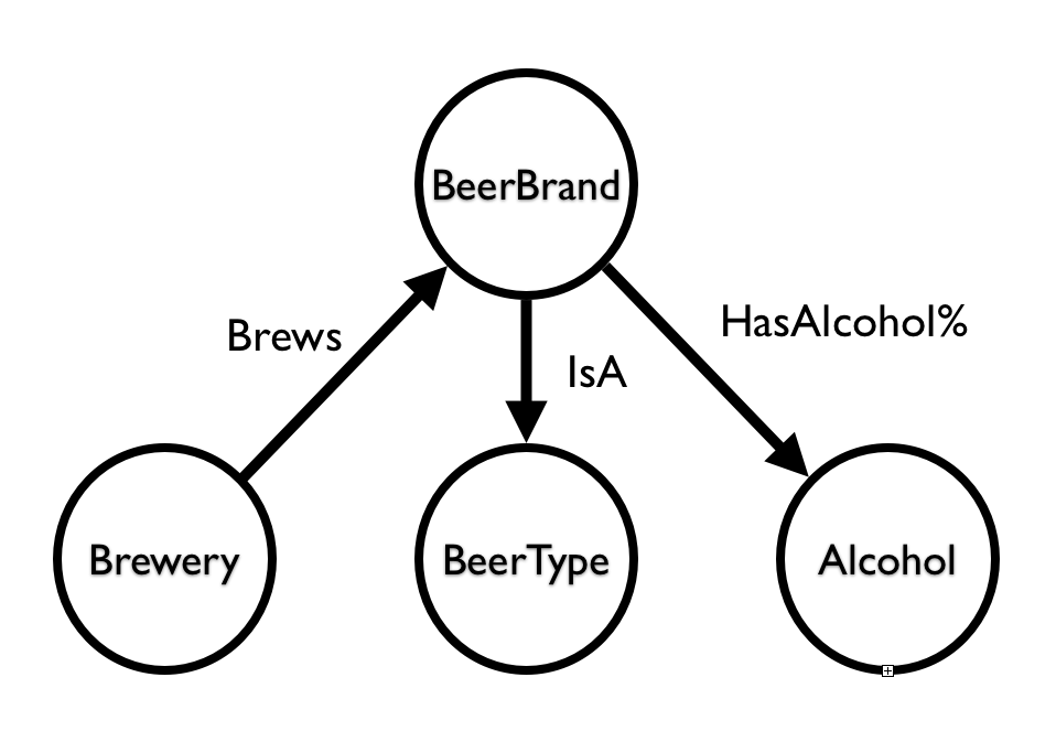
One of the things that spurred the discussion was – probably not coincidentally – the AlcoholPercentage. Many people were expecting that to be a *property* of the Beerbrand – but instead in my beergraph, I had “pulled it out”. The main reason at the time was more coincidence than anything else, but when you think of it – it’s actually a fantastic thing to “pull things out” and normalise the data model much further than you probably would in a relational model. By making the alcoholpercentage a node of its own, it allowed me to do more interesting queries and pathfinding operations – which led to interesting beer recommendations. Which is what this is all about, right?

Taking the AlcholPercentage to the next level

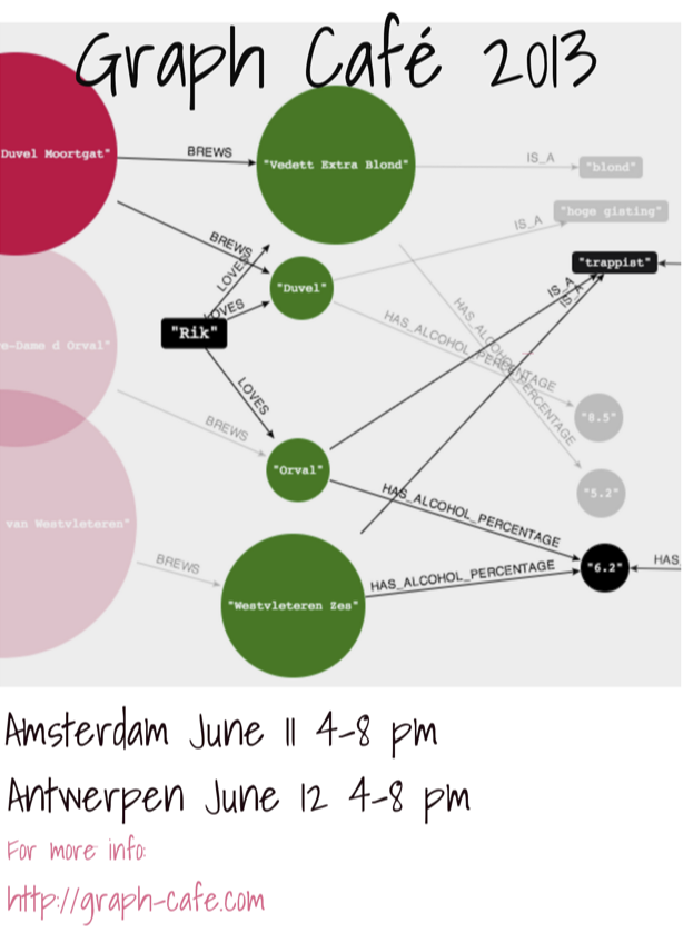
So in my new version of my beergraph, I have done something different. I used the example of Peter to create an in-graph index of AlcoholPercentages – a bit like the picture of the new model that you see here.

Essentially what I am doing is I am connecting all the alcohol-percentages into a chain of alcholpercentages – using the [:PRECEDES] relationship. In Cypher-style ascii-art that would be something like

… -(alcperc-0.2)-[:PRECEDES]->(alcperc-0.1)-[:PRECEDES]->(alcperc)-[:PRECEDES]->(alcperc+0.1)-[:PRECEDES]->(alcperc+0.2)- …

To do this, I of course did have to modify my beer-spreadsheet a little bit. You can find the new version over here. But from the screenshot below you can see that all I did was create another tab that had all the alcoholpercentages and that “PRECEDES” relationship between them. Easy peasy.

Nice. So what? The resulting dataset is very similar to what we had before – it’s just a little bit richer. You immediately notice it as you start “walking” the graph on the WebUI: the links to the AlcoholPercentage-chain gives me a new and interesting way to explore the graph.

But what else what can we do with this? Well, querying it is the obvious answer. Let me give you a couple of examples:

how can I find beers that have the same beertype and a “same or similar” alcoholprecentage (let’s say + or – 1%) as a beer that I really like (Orval). That’s now become very easy:

start

orval=node:node_auto_index(name=”Orval”)

match

orval-[:IS_A]-beertype,

orval-[:HAS_ALCOHOL_PERCENTAGE]-alcperc,

alcperc-[:PRECEDES*0..10]-otheralcperc,

otherbeer-[:HAS_ALCOHOL_PERCENTAGE]-otheralcperc,

otherbeer-[:IS_A]-beertype,

otherbeer-[:BREWS]-otherbrewery

return

otherbeer.name, beertype.name, otherbrewery.name;

Or another example:

how can I find other beers from the same brewery that have a similar AlcoholPercentage as a beer that I also like (Duvel)

start

duvel=node:node_auto_index(name=”Duvel”)

match

duvel-[:BREWS]-brewery,

duvel-[:IS_A]-beertype,

duvel-[:HAS_ALCOHOL_PERCENTAGE]-alcperc,

alcperc-[:PRECEDES*1..10]-otheralcperc,

otherbeer-[:HAS_ALCOHOL_PERCENTAGE]-otheralcperc,

otherbeer-[:IS_A]-otherbeertype,

otherbeer-[:BREWS]-brewery

return

otherbeer.name, otherbeertype.name, brewery.name,

otheralcperc.name

order by

otherbeer.name;

Both of the queries above gave me some new, interesting insights that I did not know before, allowing me to discover even more and nicer Belgian beers. But what’s important is of course that these in-graph indexes are fantastically interesting. By “pulling the data out”, normalising even further, and then indexing the normalised data as a subgraph of it’s own, we can much more easily derive new and interesting insights. And that, my dear friends, is what graphs are all about 🙂 …

Hope this was useful. If you like this post and want to discuss more about graphs and beer, please come to our Graph Café in June in Antwerp or Amsterdam – or at a pub near you?

Want to learn more about graph databases? Click below to get your free copy of O’Reilly’s Graph Databases ebook and discover how to use graph technologies for your application today.

Download My Ebook