Use Sentiment Analysis to Understand Risk Appetite

A Classic Problem Suitable for Graph Analysis

Due to its subjective and personal nature, defining and measuring risk appetite is difficult, with many often relying on “gut instinct.” A simple definition of risk appetite is “defining the level of risk an organization is willing to accept to achieve a goal.” Typically, risk appetite is scored on a 1-25 scale. But what is an acceptable risk? Critics argue that vague definitions and arbitrary numerical scoring systems are insufficient. 

So, is there a better, practical approach?

Why Define a Risk Appetite?

Why is risk appetite difficult to define? What are the challenges of defining risk appetite? What are the benefits of defining a risk appetite? 

Why is it Difficult to Define?

If we accept that “one person’s risk is another person’s opportunity,” then risk is innately personal. For example, one person may buy the lowest-priced car insurance, based on their belief that they won’t have an accident, and spending more than the minimum amount is a waste. Someone else may buy the highest-priced premium. Both approaches are reliant on the rest of the world complying. In business, being first to market and maintaining a pre-eminent position is a singular criterion. Competition is guaranteed, and success from the outset has many variables. One fundamental question for a business is, “Do we invest in product features or security?” Product features can often ensure market success. Securing the product may reduce the risk of a security incident, but at the expense of market need. This binary choice fails to recognize that business success depends on features and their secure delivery.

A decision in one context can quickly change. For example, a decision to invest in new technology may abruptly change for any number of reasons, such as the appearance of a better technology or a change in the political or financial environment. When the VCR was introduced, it was a breakthrough technology, and there were two competing solutions: VHS and Betamax. Briefly, VHS won out only to be superseded by the rise of CD/DVD. Context changes. The developments in global trading that have stood for three decades are under significant strain. Few predicted the global political, financial, business, and climatic changes of the past decade. Climate change is a good example of a growing reality, but there remain many who don’t believe in this existential risk. For many businesses, in complex and dynamic environments, attempting to define risk appetite is as much a “gut instinct” as it is measurable. 

“Gut instinct” is interesting. We all live with a level of cyber risk either directly, through our own day-to-day technology use, or indirectly, by relying on others, to protect our most precious information. This highlights a rarely acknowledged problem. For a government or commercial organization to define risk appetite has a practical impact. It creates jeopardy. In some industries, there might be concerns that a formal risk appetite statement, attributable to specific individuals, could be used in legal or regulatory proceedings; to make matters worse, this may extend to personal liability. Documenting accepting a risk of a ransomware attack, only for the criminal to then carry out a successful attack, leaves them open to the ire of both investors and customers. Defining risk appetite remains a nebulous concept, and, subconsciously, it’s not something they want to put a number on.

The Challenges of Measuring Risk Appetite

Vague definitions such as “high,” “medium,” or “low” are often used to measure risk, but they’re rarely explained well. Arbitrary numerical risk scores are created to provide a sense of a scientific approach, which the U.K. National Cyber Security Centre (NCSC) has suggested is no better than pseudoscience. The familiarity that decision-makers have with various approaches, such as “traffic light” or “5×5” matrices, normally underpinned by some numerical scoring system, because they’re “easy to understand,” makes change difficult. These all have the appearance of utility, and they’re familiar, so they make it hard for new approaches to break in.

There are some problems that lend themselves to risk. These problems are “hard.” Hard problems can be mathematically proven. For example, a structural engineer is able to understand the risk of a building falling down in an earthquake because they can model and calculate stress. Other “softer” problems are not as fortunate; for example, defining the cyber threat level and deciding on sufficient protection to combat it is full of ambiguity. For these softer issues, the psychology of risk has a tremendous impact. Risk becomes an inherently personal thing and is more about our gut instinct. This blog assumes that day-to-day risk for business decisions relates to “soft risks” and that they’re influenced by personal knowledge, experience, and sentiment.

Benefits of a Defined Risk Appetite

Despite challenges, risk guides how an organization handles financial, operational, technical, cyber, and/or reputational risk. Risk appetite that’s aligned with overall strategic goals supports effective decision-making and gives organizations the framework to manage risk at the appropriate level. Few organizations can afford for every risk decision to flow to the top. Giving people the confidence to make a decision that’s calibrated, in the context of the business, frees up decision-making and is essential to effective operations. Clearly defining risk appetite, with whatever method is used, so that everyone understands what’s acceptable, will lead to better decision-making at the appropriate level.  

The Unspoken Reality of Risk Appetite

Many organizations are reluctant, or simply don’t publish a risk appetite statement, signed off by leadership, because they tend to get on with the job regardless of any formal statements. This is instructive, as many risk managers have a good subconscious understanding of their business risk appetite simply through observing the way people behave. Leadership may not issue a formal statement of their risk appetite, but the way they behave provides insight into their appetite. I once had the unenviable task of briefing a commander on the threat to their aircraft operating in a hostile environment. The risk was helpfully described as HIGH. Talking to many people validated that there was a significant risk. Operations continued. So what’s the unspoken reality? The reality is that we often take risks based on experience, understanding, and our known capabilities, despite being told about significant risks. With hindsight, it made no difference whether the risk was defined as LOW, MEDIUM, or HIGH because other factors played a critical role in understanding capabilities: self-belief and gut instinct.

Proposed Approach

Despite years of research and application, understanding organizational risk is problematic. Old, familiar tools continue to be used and, in many cases, are an exercise in process that more often than not is ignored when reality kicks in. We will assume that we’ve rejected the traditional approaches to defining risk appetite, as in publishing a formal statement. Instead, we’ll use behavior and attitude captured through a series of questions to calculate a risk appetite score. This isn’t perfect, but it may more accurately reflect organizational, and specifically leadership behavior, and act as a more effective guide as to how risk is managed in an organization. The next section describes how, using graph database tools, we can provide this insight.

The Risk Appetite Calculation Method

Approach

We propose using three question sets, structured differently, progressively giving the respondent freedom to respond. A combination of multiple choice and free response allows for calibration. The multiple-choice and free-response questions will be handled differently in the analysis to help develop a view of the appetite.

Multiple Choice

Ideally, we would have labeled data to train a model on (i.e., a set of answers to our multiple-choice questions labeled with corresponding risk appetites). Since this doesn’t exist, we have to consider ways around this.

The first option relies on the fact that the multiple-choice questions have “obvious” more risky and less risky answers. This allows us to collect a large sample of responses to the questions and use these to work out what fraction of the population chooses each answer. We can then formulate statements like, “If a user chooses option A, they’re more risky than 70 percent of the population.” This option has the advantage of using a large sample of data, which means the calculated risk appetite is directly comparable to real people, so we may be able to say that a user is in a certain percentile of risk-takers. 

Collecting data raises many problems:

• It’s expensive and time-consuming
• Which population do we collect data from?
• How do we minimize bias in our data collection?
• How do we sample the population to ensure that participants represent the variety of characteristics, roles, and views present in the population?

This approach raises another question: After collecting data and performing a calculation that places a user in a certain risk percentile, how do we convert this to 1-25 score that is comparable to a risk severity score? It isn’t as simple as a linear conversion. This would imply that the population is spread evenly across the scale from 1 to 25, but it’s more likely that you would have a large majority of people close to the average risk appetite, with very few holding an extreme risk appetite. You now need to consider what the average risk appetite is and what the variation is among the population.

The second option relies on eliciting expert knowledge rather than collecting data. This option is much faster and cheaper, but raises the problem that it’s often challenging to get an expert to convert their knowledge into quantitative values. 

There are many ways to approach turning expert knowledge into useful data. We’ll use the approach of getting the expert to answer the multiple-choice questions from the perspective of different risk appetites (e.g., 5, 10, 15, 20). It’s important that when doing this, the expert closely references the business methodology used to classify the impact and probability of a risk. The idea is to minimize the expert’s opinion but use their expertise to classify the impact and probability of each situation.

The disadvantages of this approach stem from the expert’s subjectivity. Subconscious biases cannot be removed and will affect the way the expert answers the questions. This will then affect the appetite score assigned to each user. 

Free Response

The objective of analyzing the free-response answers is to translate the sentiment of the response to a risk appetite. 

One approach is to use existing sentiment analysis tools to analyze responses. Most sentiment analysis tools are designed to give output based on how positive, negative, or neutral the input is, which is a problem because it doesn’t necessarily align with the underlying risk in the answer (i.e., it’s possible to give two answers, both of which are positive, but one is risky and the other is cautious). Sentiment analysis tools are also often context-specific; for example, many tools are trained to determine whether a product review is positive or negative and wouldn’t work well outside of this context. To use such a sentiment analysis tool, a custom tool would need to be trained on relevant labeled text data.

Another common approach to representing text data is to use vector embeddings, which allows the texts to be represented as vectors that can then be more easily compared. These vector embeddings could then be used in a similar way as the multiple-choice responses, where they are compared to existing “model answers” from different risk appetites. This approach has two main problems: You would need to create a large set of model answers to compare the vector embeddings against, and vector embeddings capture more than the underlying risk sentiment in each text, so similarity between vector embeddings doesn’t necessarily imply similar risk appetites.

The third approach is to use a large language model (LLM) to capture the risk appetite behind each response. This would involve engineering an appropriate prompt to get the LLM to produce a risk appetite score when given a question and response. Using an LLM has two main benefits. An LLM can be fed a huge amount of context, which can include almost anything relevant to the business, but it should definitely include the methodology of how the impact and probability of risks are classified. The second benefit comes from giving the LLM the methodology of classifying impact and probability which means the LLM can respond with an exact risk appetite score that directly aligns with how risks are classified. However, out of the three approaches, this one is the biggest “black box,” and using AI for a consequential decision may leave a bad taste.

The Recommended Approach

Due to the cost and time delay in collecting data, it’s recommended to rely on expert knowledge to solve for the lack of labeled data. The expert in this case may be anyone suitably experienced in risk management — for example, the Governance, Risk, and Compliance (GRC) staff, business risk manager, or the CISO. Ideally, this expert shouldn’t be part of the group whose responses will be used to calculate the risk appetite score.

It’s important to consider how we’re going to use this newly labeled data. In the approach detailed later, we’ll find which risk profile shares the most answers with each user and assign the user that risk appetite. If we aren’t careful, we may end up in a situation where two risk profiles share similar answers. To make this approach as fair as possible, we should have close to an equal number of different answers for each risk profile. This may take some tuning to select appropriate questions and possibly removing questions where all risk profiles have the same answer. The question sets also need to be developed for each organization because one size doesn’t fit all.

When considering the approaches to the free-response questions, both using existing sentiment analysis tools and vector embeddings suffer from the problem that they don’t exactly capture the underlying sentiment. While developing a custom sentiment analysis tool trained on relevant text data may be the best solution, it’s outside the scope of this problem. The use of an LLM has one major advantage over the other options that makes it the favorable choice: the ability to give the context of how risks are classified. Since a large use of a risk appetite score is to be able to compare it against risks, it’s important that they’re both measured against the same scale. 

Measuring Risk Appetite

This section outlines a suggested approach to defining organizational risk appetite. 

Objective

Our aim is to use responses to a set of multiple-choice and free-response questions to calculate a risk appetite. Risk appetite was defined earlier as “the level of risk an organization is willing to accept to achieve a goal,” so our risk appetite needs to be on the same scale used to classify risks so we can compare the two. We assume a  5×5 probability and impact matrix is used to classify risks, which is then used to calculate severity = impact probability. This means severity ranges 1-25, so our risk appetite should be a number in that range. 

Assumptions

Risk matrices and, in particular, severity scores have a significant incorrect underlying assumption. This assumption is that as impact and probability are assigned numeric scores (i.e., 1-5), they can be treated as numeric variables. Impact and probability ratings are in fact ordinal categorical variables, which leads to many incorrect interpretations.

Numeric variables represent measurable quantities (e.g., height, weight, or age), so it makes sense to perform calculations using these values. Categorical variables fall into categories, such as eye color or marital status. Ordinal categorical variables are categorical variables that give way to an ordering or ranking, such as exam results where A>B>C. Although ordinal categorical variables can be ordered, it wouldn’t make sense to perform calculations (e.g., A-B is nonsensical). In our case, impact rating and probability are actually ordinal categorical variables, although they’re misleadingly labeled 1-5, causing people to treat them as numeric.

As discussed, it doesn’t make sense to use categorical variables in calculations, so the calculation of severity = impact x probability is less meaningful than at first glance. This can be seen by considering a risk of impact 5 and probability 1 against a risk of impact 1 and probability 5. Most people would likely have a strong preference for which risk they would rather accept, and yet using the severity rating, they’re exactly the same. Risks should really be classified into 25 unique categories, one for each pair of impact and probability ratings. This severity calculation causes trouble when trying to calculate a risk appetite to compare against it.

Approach

This section will cover the details behind the calculation using the recommended approach. Collecting and writing the data to the database won’t be covered in detail here, as extensive documentation already exists on this. One approach that can be implemented quickly is to use a Google form to collect CSV data and use APOC load procedures to write this data to the database.

While we won’t cover how to upload the data, we’ll briefly mention the schema used when storing the data. The “Type” of the question will denote whether it’s multiple choice or free response because it’s necessary to differentiate between how we treat these questions. 

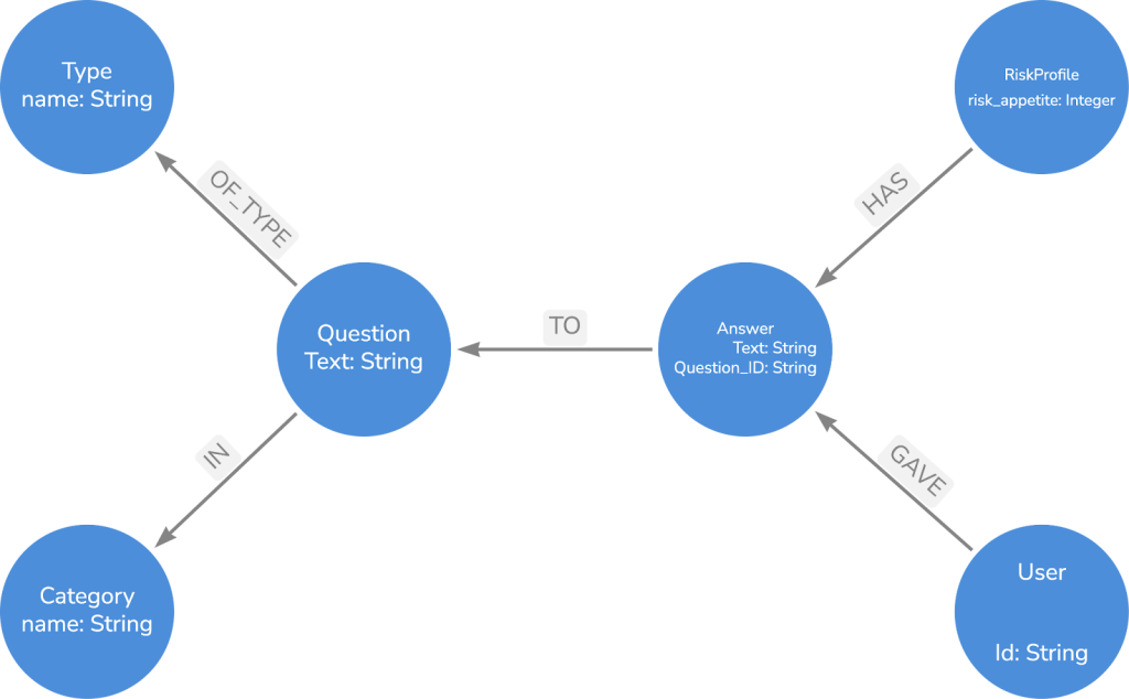
The risk profile seen here refers to the approach used for the multiple-choice questions in which an expert would answer the questions from the perspective of different risk profiles or appetites. So each risk profile is assigned the risk appetite it represents. We won’t use the category node directly in any of the calculations, but it may be of some interest to have a separate risk appetite for different categories.

You may notice that the answer nodes have a question ID property. This is to ensure that answer nodes aren’t shared between questions. For example, the answers “yes” and “no” may be repeated many times, but we don’t want them to have a relationship to many question nodes because it would be impossible to differentiate which user gave which answer to which question.

After importing the data, we can now look at the Cypher necessary to complete the calculation. For the first part of the calculation, we want to compare users’ answers to the risk profiles. We’ll do this by simply finding the risk profile that shares the most answers with a user. This is a simplified version of the nearest-neighbor approach, and by finding the risk profile with the greatest overlap, we’re really finding the risk profile with the shortest Hamming distance to each user. In the rest of the calculation, we assume that we’ll simply assign the user the risk appetite of the closest risk profile. However, you may want to find multiple nearest risk profiles and calculate risk appetite by performing a weighted average of the nearest risk appetites, where the weights are based on the number of answers shared.

Below is an example Cypher query used to find the closest risk appetite for each user. For each user, it matches all of the shared answers with each risk profile, then for each risk profile, it counts the number of overlaps. ORDER BY is used to find the risk profile with the greatest overlap. The second part of the ORDER BY line is used as a tie-breaker. In this case, it simply chooses whatever risk appetite is closer to 13.

  MATCH (u:User)
  WITH u
  CALL(u){
    MATCH (u)-[:GAVE]->(a:Answer)<-[:HAS]-(rp:RiskProfile)
    WITH rp, count(a) AS overlap
    ORDER BY overlap DESC, abs(rp.risk_appetite - 13) ASC LIMIT 1
    RETURN rp
  }
RETURN u, rp

The second part of the calculation using an LLM requires slightly more configuration. In this example, we will use the OpenAI chat completions API. Below is the subquery used on every free-response question and answer. It consists of configuring the payload and using apoc.load.jsonParams.

 CALL(user_prompt, system_prompt){
    WITH "https://api.openai.com/v1/chat/completions" AS url,
     { 
       Authorization: "Bearer " + $openai_token, 
       `Content-Type`: "application/json" 
     } AS headers,
     apoc.convert.toJson({
       model: "gpt-4.1",
       temperature: 0.0,
       messages: [
         { role: "system", content: system_prompt},
         { role: "user", content: user_prompt }
       ]
     }) AS payload
    CALL apoc.load.jsonParams(url, headers, payload, null) 
    YIELD value
    RETURN toInteger(value.choices[0].message.content) AS response
    }

This subquery takes two parameters: a system prompt and a user prompt. These are passed under “messages.” The system role is used to define the highest-priority instructions. If there’s anything in the user prompt that conflicts with the system prompt, the system prompt overrules the user prompt. 

The system prompt is used to define the task we want the LLM to complete, and the user prompt feeds both the question and response we want the LLM to produce a risk appetite score for. The system prompt must be specific to each business, but there are some main areas the prompt should cover:

• A description of the task requirements (producing a risk appetite score based on a user’s response to a question).
• Context – most importantly, the guidelines for how risks are classified, any information about the business, such as the products and services it provides and the industry it operates in, will help produce a more relevant appetite score.
• Tuning – You may find it useful to provide an expected average risk value or some description of the variation of appetites (for example, 90 percent of scores should fall between 5 and 20).
• Formatting – Since the output is used in the rest of the calculation, the output needs to be formatted to return only a float or integer.

After the calculator for both the multiple choice and free response is completed, you need to consider how to combine them. It may be as simple as finding their average, but you may want to weigh one more importantly than the other. This can even be taken as far as giving weights to individual questions.

Challenges

The biggest challenge in this calculation is the subjectivity of risk. No matter how objective you try to make your risk assessment methodology, people’s subconscious biases will affect the outcome. So while this risk appetite score is useful, it must be taken with a pinch of salt. The risk appetite score shouldn’t necessarily be used as a hard and fast rule to decide which risks should be accepted, but rather as a tool to help risk management. The risk appetite could be best used as a benchmark against which to compare the average risk the business is taking on or, more importantly, the number of risks that are above the risk appetite.

There are inherent difficulties in defining and measuring risk appetite due to its subjective and personal nature. With so much variance, it can be a challenge to determine. We’ve shown a few approaches and techniques to take the guesswork out of it.