From Nodes to Rows: A Guide to Querying Neo4j Graph Database in Pandas/SQL Style Using Cypher

Well, you might be wondering: Why would one want to write Pandas or SQL-style queries while working with a graph database like Neo4j? Does it not defeat the purpose of having data stored and ingested in a graph DB in the first place? No, it doesn’t.

Graph databases excel at storing and querying complex, connected data that is difficult to represent in a traditional tabular database. However, not all data analysts/scientists who wish to analyze a graph database are fluent in Cypher, the query language used by many graph databases.

They may be more comfortable performing data analysis in SQL or Pandas, and wish to perform tabular-style data analysis on a graph. In such cases, writing SQL or pandas-style queries in Cypher provides a way to leverage the benefits of the graph database while working within a familiar framework.

Additionally, there may be a need to first perform exploratory data analysis in SQL or pandas before leveraging the graph structure to gain additional insights.

For instance, suppose you have a graph database with millions of nodes and relationships, and you need to perform data analysis or visualization tasks that require working with tabular data. In that case, you can use pandas-style queries to extract data from the graph database and manipulate it in a way that’s more suitable for your needs.

This can help you gain a better understanding of the data and uncover patterns or relationships that may not be immediately apparent from a graph structure. Once you have extracted the necessary data, you can use it to make informed decisions about how to interact with the original graph database.

Therefore, pandas or SQL-style queries in Cypher do not defeat the purpose of using a graph database. Instead, they provide a way to work with graph data in a more flexible and convenient way, without sacrificing the benefits of using a graph database.

Now, let’s get to the fun part — writing Cypher queries for common analysis operations performed on tabular data. We will be running queries on the sample Northwind Graph provided by Neo4j for exploration purposes.

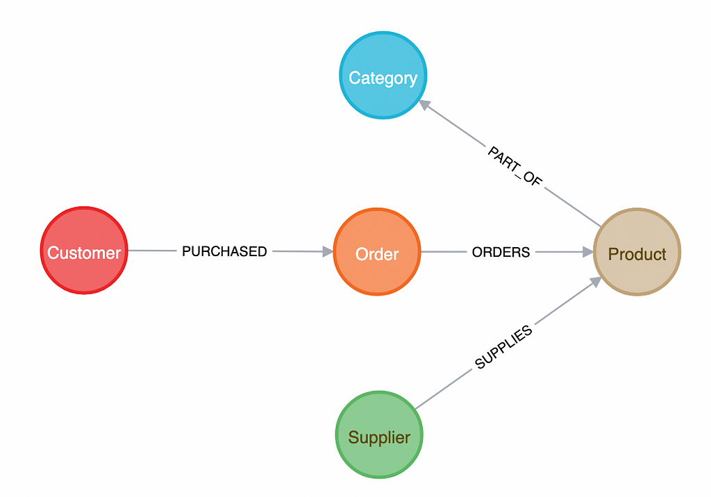
To load this dataset into Neo4j please follow the instructions here: https://development.neo4j.dev/graphgists/northwind-recommendation-engine/.

To run the pandas code, I used the dataset available here: https://github.com/graphql-compose/graphql-compose-examples/tree/master/examples/northwind/data/csv.

[Note by Publication] There is a dedicated graph example dataset for Northwind available here:

GitHub – neo4j-graph-examples/northwind: From RDBMS to Graph, using a classic dataset

1. Getting value counts of a list of values:

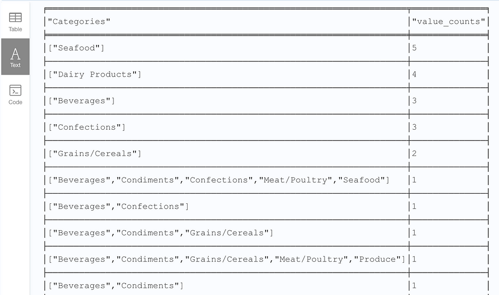
Sample Question: List the counts of the unique list of product categories provided by each supplier.

Pandas equivalent code:

# read the data from the CSV files
categories = pd.read_csv('https://raw.githubusercontent.com/graphql-compose/graphql-compose-examples/master/examples/northwind/data/csv/categories.csv')
products = pd.read_csv('https://raw.githubusercontent.com/graphql-compose/graphql-compose-examples/master/examples/northwind/data/csv/products.csv')
suppliers = pd.read_csv('https://raw.githubusercontent.com/graphql-compose/graphql-compose-examples/master/examples/northwind/data/csv/suppliers.csv')

# merge the dataframes on the necessary columns
merged = pd.merge(pd.merge(products, categories, on='categoryID'), suppliers, on='supplierID')

# group by supplier and category and count the occurrences
merged_groupby = merged.groupby(['companyName'])['categoryName'].unique().reset_index()

# display the results
print(merged_groupby['categoryName'].value_counts())

SQL equivalent query (if data was stored in a relational DB):

SELECT array_agg(DISTINCT c.categoryName) AS Categories, COUNT(*) AS value_counts
FROM supplier s
JOIN product p ON s.supplierID = p.supplierID
JOIN category c ON p.categoryID = c.categoryID
GROUP BY s.companyName
ORDER BY value_counts DESC;

Cypher query:

MATCH (s:Supplier)-->(:Product)-->(c:Category)
WITH s.companyName as Company, collect(distinct c.categoryName) as Categories
RETURN Categories, COUNT(*) AS value_counts
ORDER BY value_counts DESC

If we just wanted the categories as a list (this query is already given in part 4/7 of the playbook), the query would be:

MATCH (s:Supplier)-->(:Product)-->(c:Category)
RETURN s.companyName as Company, collect(distinct c.categoryName) as Categories

However, to get the value counts of an array, the simple trick is to first write a query to return the array, and then change the RETURN to WITH. Then add a return statement to treat this array as a single entity and just do a COUNT(*). Also, notice how we can easily perform multiple joins in just one MATCH line in Cypher.

Cypher output:

2. Joining, grouping, and aggregating data:

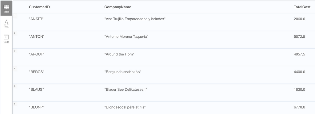
Sample Question: Which customers have made orders with a total cost greater than $1000?

Pandas equivalent code:

# read the data into pandas dataframes
products = pd.read_csv('https://raw.githubusercontent.com/graphql-compose/graphql-compose-examples/master/examples/northwind/data/csv/products.csv')
order_details = pd.read_csv('https://raw.githubusercontent.com/graphql-compose/graphql-compose-examples/master/examples/northwind/data/csv/order_details.csv')
orders = pd.read_csv('https://raw.githubusercontent.com/graphql-compose/graphql-compose-examples/master/examples/northwind/data/csv/orders.csv')
customers = pd.read_csv('https://raw.githubusercontent.com/graphql-compose/graphql-compose-examples/master/examples/northwind/data/csv/customers.csv')

# merge the dataframes on common columns
merged_data = pd.merge(pd.merge(order_details, orders, on='orderID'), products, on='productID')
merged_data = pd.merge(customers, merged_data, on='customerID')

# calculate the total cost for each order
merged_data['totalCost'] = merged_data['unitPrice_x'] * merged_data['unitsOnOrder']

# group the data by customer and sum the total cost
customer_order_totals = merged_data.groupby(['customerID','companyName']).agg({'totalCost': 'sum'})

# filter for customers with total cost greater than $1000
high_spending_customers = customer_order_totals[customer_order_totals['totalCost'] > 1000]

# print the list of high spending customers
print(high_spending_customers)

SQL equivalent query (if data was stored in a relational DB):

SELECT CustomerID, CompanyName, TotalCost
FROM (
  SELECT c.CustomerID AS CustomerID, c.CompanyName AS CompanyName, SUM(p.UnitPrice * p.UnitsOnOrder) AS TotalCost
  FROM Customers c
  JOIN Orders o ON c.CustomerID = o.CustomerID
  JOIN `Order Details` od ON o.OrderID = od.OrderID
  JOIN Products p ON od.ProductID = p.ProductID
  GROUP BY c.CustomerID, c.CompanyName
  HAVING TotalCost > 1000
) t;

Cypher query:

MATCH (c:Customer)-[:PURCHASED]->(o:Order)-[:ORDERS]->(p:Product)
WITH c, SUM(p.unitPrice * p.unitsOnOrder) AS TotalCost
WHERE TotalCost > 1000
RETURN c.customerID AS CustomerID, c.companyName AS CompanyName, TotalCost

Again, notice how we can easily perform multiple joins in just one MATCH line in Cypher.

In this query, we first connect the data belonging to all the relevant nodes, i.e., products, categories, orders, and customers. Then, we group the data by category and calculate the total revenue generated by summing up the product of the quantity and unit price for each order.

Cypher output:

3. Filtering using negation of subquery:

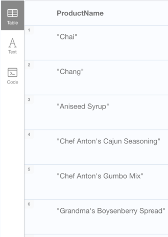
Sample Question: What are the product names of all products that have not been ordered by customers from Germany?

Pandas equivalent code:

# read the data from the CSV files
orders = pd.read_csv('https://raw.githubusercontent.com/graphql-compose/graphql-compose-examples/master/examples/northwind/data/csv/orders.csv')
customers = pd.read_csv('https://raw.githubusercontent.com/graphql-compose/graphql-compose-examples/master/examples/northwind/data/csv/customers.csv')
products = pd.read_csv('https://raw.githubusercontent.com/graphql-compose/graphql-compose-examples/master/examples/northwind/data/csv/products.csv')
order_details = pd.read_csv('https://raw.githubusercontent.com/graphql-compose/graphql-compose-examples/master/examples/northwind/data/csv/order_details.csv')

# merge the dataframes on the necessary columns
merged = pd.merge(pd.merge(pd.merge(products, order_details, on='productID'), orders, on='orderID'), customers, on='customerID')

# find the product names not ordered by customers from Germany
not_ordered_by_germany = merged[merged['country'] != 'Germany']['productName'].unique()

# filter the products dataframe to get the product names
result = products[products['productName'].isin(not_ordered_by_germany)]['productName']

# display the results
print(result)

SQL equivalent query (if data was stored in a relational DB):

SELECT productName
FROM Product
WHERE productName NOT IN (
  SELECT p.productName
  FROM Product p
  JOIN Orders o ON p.productId = o.productId
  JOIN Customer c ON o.customerId = c.customerId
  WHERE c.Country = 'Germany'
)

Cypher query:

Version 1: Subquery style using CALL and WHERE NOT {}

CALL {
  MATCH (p:Product)
  WHERE (p)<-[:ORDERS]-(:Order)<-[:PURCHASED]->(:Customer {Country: 'Germany'})
  RETURN collect(p.productName) AS productName_list
}
MATCH (p:Product)
WHERE NOT p.productName IN productName_list
RETURN p.productName AS ProductName

Version 2: Concise without CALL {} subquery.

MATCH (p:Product)
WHERE NOT exists {(p)<-[:ORDERS]-(:Order)<-[:PURCHASED]->(:Customer {Country: 'Germany'}) }
RETURN p.productName  AS ProductName

Again, notice how we can easily perform multiple joins in just one MATCH line in Cypher. Furthermore, we can see that using CALL{} to write a subquery-style query in Cypher while being a valid option, is not necessary. It may be possible to make the query even more concise without an explicit subquery.

Cypher output:

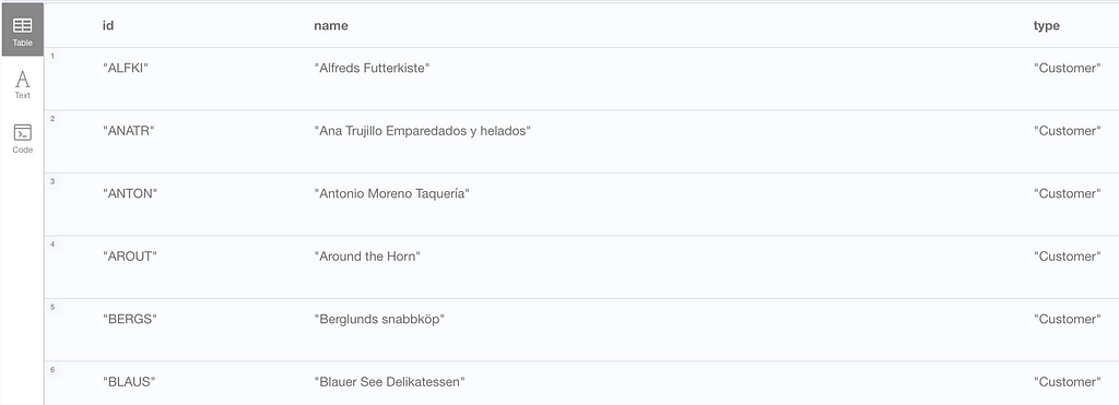
4. Concatenating data (vertically):

Sample Question: List all customers and suppliers in one combined list with their respective names and types of entity.

Pandas equivalent code:

# Define data for Customers
customers = pd.read_csv('https://raw.githubusercontent.com/graphql-compose/graphql-compose-examples/master/examples/northwind/data/csv/customers.csv')

customers['type'] = 'Customer'
customers = customers.rename(columns={'customerID': 'id', 'companyName': 'name'})
customers = customers[['id', 'name', 'type']]

# Define data for Suppliers
suppliers = customers = pd.read_csv('https://raw.githubusercontent.com/graphql-compose/graphql-compose-examples/master/examples/northwind/data/csv/suppliers.csv')

suppliers['type'] = 'Supplier'
suppliers = suppliers.rename(columns={'supplierID': 'id', 'companyName': 'name'})
suppliers = suppliers[['id', 'name', 'type']]

# Concatenate data
result = pd.concat([customers, suppliers], ignore_index=True)

# display the results
print(result)

SQL equivalent query (if data was stored in a relational DB):

SELECT customerID AS id, companyName AS name, 'Customer' AS type
FROM Customers
UNION ALL
SELECT supplierID AS id, companyName AS name, 'Supplier' AS type
FROM Suppliers;

Cypher query:

MATCH (c:Customer)
RETURN c.customerID AS id, c.companyName AS name, 'Customer' AS type
UNION ALL
MATCH (s:Supplier)
RETURN s.supplierID AS id, s.companyName AS name, 'Supplier' AS type

In this case, both the SQL and Cypher queries are very similar with only minor syntax differences. However, the Pandas version is a bit more verbose.

Cypher output:

Takeaways:

We can perform the same data analysis that we do using Pandas or SQL , using Cypher queries as well, if the data is loaded into Neo4j in the right way. It is not necessary that Cypher queries are always simpler than their equivalent Pandas code or SQL queries, but many times, they indeed might be.

This is because of the following advantages of querying using Cypher:

1. Easier joins: Connecting data is generally easier in Cypher as compared to SQL because Cypher is specifically designed for querying graph patterns and focuses on the relationships between nodes rather than just the properties of nodes.
   In Cypher, we can traverse the graph and follow relationships to join different nodes together, which is a more natural and intuitive way of joining data when working with graphs. On the other hand, in SQL, joining data involves a lot of complex syntaxes and can be challenging to understand.
2. Flexible pattern matching: Another advantage of Cypher is that it allows for easier pattern matching. You can use the MATCH clause to specify the nodes and relationships you’re interested in, and then use the WHERE clause to filter the results.
   This can be more flexible than SQL, which requires you to specify the exact columns and tables you want to query. With Cypher, you can focus on the patterns in the data and write queries that capture them more easily.

However, it is important to keep in mind that using a graph DB like Neo4j to store and query your data might not be the best choice in all scenarios, especially when data is more structured and less interconnected relationships.

But, if your data has complex relationships, and you need to perform complex queries, scale your analysis, or want greater flexibility in your data modeling, then, a graph database like Neo4j would likely be a better choice than a relational database.

Writing queries in Cypher might be uncomfortable to begin with, but practicing regularly will make you confident in your Cypher data analysis skills in no time. GraphAcademy courses are a great place to learn Neo4j, with their amazing hands-on in-built exercises.
I personally used these a lot on my Cypher learning journey.

Thank you for reading my article. If you liked this article, and wish to see more such content, please show some support by following me on Medium.

If you would like more specific content on Neo4j or any other graph DB, please comment below with details. Cheers!

From Nodes to Rows: A Guide to Querying Neo4j Graph Database in Pandas/SQL Style Using Cypher was originally published in Neo4j Developer Blog on Medium, where people are continuing the conversation by highlighting and responding to this story.