Topic Extraction with Neo4j GDS for Better Semantic Search in RAG Applications

Senior Data Scientist at Neo4j
17 min read
Semantic search allows search systems to retrieve documents that match the meaning of a query even if the exact keywords in the query are not present in the document. This flexible retrieval capability is a key part of many Retrieval Augmented Generation (RAG) applications in Generative AI.
RAG applications use semantic search to find relevant documents and then ask a Large Language Model to answer questions based on the documents retrieved.
Semantic search depends on summaries of text documents in the form of numeric vectors. These vectors are stored in a vector store, like Neo4j. At query time, a user’s query is converted to a vector, and the documents from the vector store with the most similar vector representations are returned.
There is some art to breaking down long documents into smaller chunks for vector summarization. If the chunks are too large, the vector summary could fail to highlight minor themes in the document that might be relevant to the user’s question. If the chunks are too small, a context that is important to answering the user’s questions might be fragmented across multiple text chunks.
One solution to this problem is to extract topics from documents and use them as the basis for semantic search. Once the topics most similar to a user’s question are discovered in the vector store, all documents that reference those topics can be retrieved.
Neo4j provides a rich toolset for topic-based semantic search. The Neo4j graph database platform allows us to represent documents and related topics as a knowledge graph. Neo4j’s vector search capability enables semantic search over vector representations of topics and documents. With Neo4j Graph Data Science (GDS), we can use graph algorithms to identify and merge duplicated topics, making our searches more efficient.
In a database containing movie plots, I found that performing semantic search with graph-based topic clusters gave me 27% more relevant documents than performing semantic search on the base documents alone.
A Dataset of Recent Movies
I chose to test topic modeling for semantic search on movie information that I downloaded from TMDB.org and loaded into a Neo4j AuraDS graph database. I limited the dataset to titles released after September 1, 2023. That release date was later than the training cutoff date for the Large Language Models I used for my project. That way, I could be sure that the LLMs were using data retrieved from the Neo4j to describe the movies, not information the LLMs might have learned about the movies from their training data. The movies in the dataset included everything from Oscar-winning features to short films produced by students.
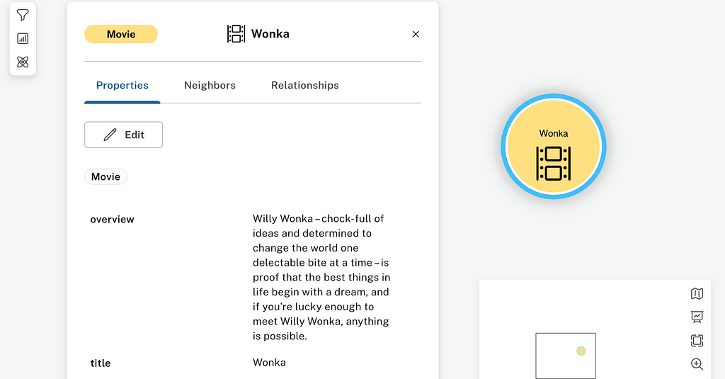
The resulting data set had 16,156 Movie nodes. Each node has a title property and an overview property containing a summary of the movie’s plot. The code that I used to load the movies to Neo4j is in the Dowload_TMDB_movies.ipynb notebook in the project repository.

Using an LLM to Extract Themes
After loading the movie data to Neo4j, I asked an LLM to find key themes in the movie title and overview. The themes might refer to specific objects, settings, or ideas. I was looking for hooks that people might think about when they searched for the move. Because I didn’t try to classify what type of theme was discovered, the task was somewhat simpler than traditional Named Entity Recognition (ER) where an algorithm tries to identify entities of specific types like dates, people, or organizations.
Here is the prompt that I used:
You are a movie expert.
You are given the tile and overview of the plot of a movie.
Summarize the most memorable themes, settings, and public figures in the movie
into a list of up to eight one-to-two word phrases.
Only include the names of people if the person is a famous public figure.
Prioritize any phrases that appear in the movie's title.
You can provide fewer than eight phrases.
Return the phrases as a pipe separated list.
Return only the list without a heading.
I used the Anthropic’s Claude 3 Sonnet model for this extraction because I had been looking for an opportunity to try their recently released models. I think other Large Language Models would do a good job at this task, too.
Here’s an example of the input I sent the model:
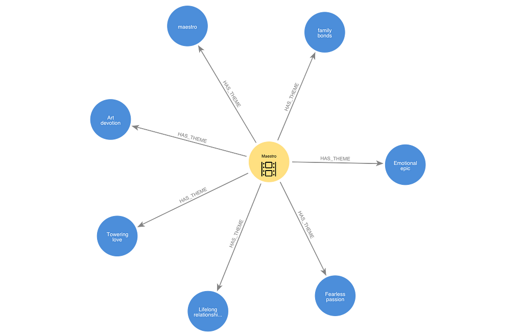
title: Maestro
overview: A towering and fearless love story chronicling the lifelong
relationship between Leonard Bernstein and Felicia Montealegre Cohn Bernstein.
A love letter to life and art, Maestro at its core is an emotionally epic
portrayal of family and love.
Here is what the LLM gave me back:
meastro|family bonds|Emotional epic|Fearless passion|Lifelong relationship|
Towering love|Art devition
I turned these responses from the LLM into Theme nodes connected to Movie nodes by HAS_THEME relationships in Neo4j.
The notebook Extract themes.ipynb in the project repository contains the code for this step of the process.
Clean up Themes and Generate Text Embeddings
The LLM did not do a perfect job of returning only a pipe-delimited list of themes. In a few cases, the list was prefixed with some extra text like “The memorable themes, settings, and public figures in this movie are:…”. In some cases, the LLM couldn’t find any themes, and it returned a sentence saying so instead of an empty list. In a few cases, the LLM decided that the content described in the overview was too sensitive or explicit to summarize. You can find the code I used to clean up these responses in the notebook Clean up themes and get embeddings.ipynb in the project repository. Because of the unpredictable nature of LLMs, you might need to take slightly different steps to clean up your themes if you run the code.
After cleaning up the themes, I used OpenAI’s text-embedding-3-small model to generate embedding vectors for the themes. I stored these vectors as properties on the Theme nodes in Neo4j. I also generated embeddings for strings that contained the movie title concatenated with the movie overview. These embeddings were stored as properties on the Movie nodes in Neo4j.
I created Neo4j vector indexes for the Theme vectors and the Movie vectors. These indexes allowed me to efficiently find the nodes with the most similar embedding vectors based on cosine similarity to a query vector that I would provide.
Cluster Themes Using Neo4j Graph Data Science
LLMs do an amazing job at manipulating language, but it is hard to get them to standardize their output. I found that the LLM identified some themes that were close synonyms. I hoped that I could make the semantic search of the themes more efficient by combining duplicated or very closely related themes. All of the code for clustering and deduplicating themes is contained in the Cluster themes.ipynb notebook in the project repository.
Use Traditional NLP Techniques to Find Themes That Share Stems
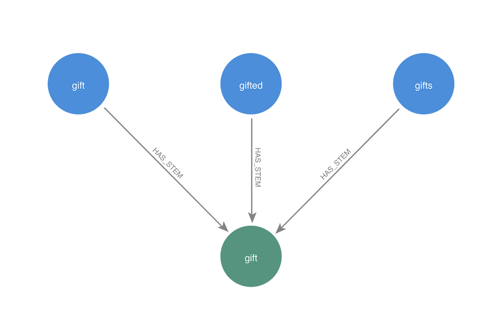
I started by using a traditional natural language processing technique to identify words that are based on the same root word, called a stem. I used the WordNet lemmatizer from the NLTK Python package to trim off prefixes and suffixes from themes to find common root words. I created Stem nodes in the graph linked them to themes with HAS_STEM relationships. I assigned the embedding vector from the Theme node in the stem group that was attached to the most Movie nodes as the embedding vector for the Stem node.
Explore similar themes that don’t share stems
There were other groups’ themes in the graph with very similar meanings, even though they didn’t share a stem. To begin to identify them, I selected some Theme nodes from the graph and ran queries against the vector index to find the other Theme nodes with the most similar embeddings. I was trying to find a reasonable cutoff for cosine similarity below, which is probably not a synonym of the two themes. I also was trying to find a cutoff for the number of close synonyms that a theme might have in the dataset.
Here’s an example of the theme “underwater”:
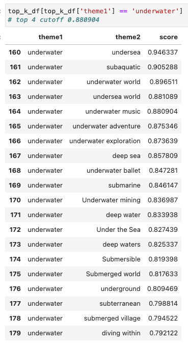
I thought “undersea,” “subaquatic,” “underwater world,” and “undersea world” were all essentially the same thing as “underwater.” The “underwater music” theme starts to introduce a new idea that I would want to preserve as a separate theme. A similarity cutoff above 0.880904 or a top k less than or equal to 4 would exclude themes that should not be lumped in with “underwater.”
Here’s the first part of the table for “fast food.”
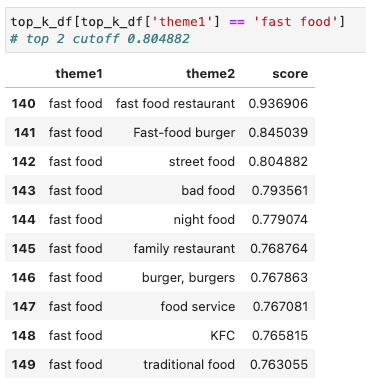
I thought the first two themes of “fast food restaurant”, “Fast-food burger” are closely enough related to be one concept. The “street food” theme seems like it deserves a different group. A similarity cutoff above 0.804882 or a top k less than or equal to 2 would preserve the distinction between street food and fast food.
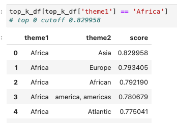
The most similar theme for “Africa” was “Asia” — a completely different continent. I would need a similarity cutoff above 0.829958 to ensure that these two themes can’t be merged in a cluster.
Create IS_SIMILAR Relationships With the K Nearest Neighbors Algorithm
After looking at the similarity for several other themes, I decided to use a similarity cutoff of 0.83 and a top k of 2. I created a graph projection that included the Stem nodes as well as all the Theme nodes that were not related to Stems. Then, I ran the K Nearest Neighbors algorithm to mutate the graph projection by adding IS_SIMILAR relationships between nodes whose cosine similarity was above the similarity cutoff and top k thresholds that I selected.
Test Weakly Connected Components Communities
The Weakly Connected Components community detection algorithm assigns any nodes that are connected by an undirected path to the same component. If I had selected very strict criteria when I created IS_SIMILAR relationships, WCC might have been a workable approach to identifying clusters of synonyms. We could make a transitive assumption that if A is a synonym of B and B is a synonym of C, then A is a synonym of C.
I ran WCC and found that the results were not ideal. I tried setting the WCC similarity threshold to 0.875, which was higher than the cutoff I used for KNN. I wanted to make sure that only very closely related themes were lumped together. The largest WCC community contained 29 themes. All of them had something to do with Christmas, but “Christmas terror” and Christmas magic” are probably going to relate to movies with very different vibes.

The other problem with setting a high similarity cutoff like 0.875 was that themes like “arid landscape” and “desolate landscape” — which I think belong together — ended up in different communities. Instead of WCC, I decided to try the Leiden community detection algorithm.
Leiden Communities Can Be Tuned for Larger or Smaller Communities
The Leiden community detection algorithm identifies communities within the graph where the fraction of the community’s relationships that start and end within the community is higher than we would expect if the relationships were distributed at random.
A parameter called gamma can be tuned to make Leiden produce a larger or smaller number of communities. I think of gamma as specifying how much more interconnected a group of nodes labeled as a community must be than what we would expect if relationships were distributed at random. As gamma increases, the cluster definition criteria become more strict. At high gamma values, large, loosely connected communities don’t pass the criteria, and small, densely connected communities remain.
Before I could run Leiden, I needed to modify the graph projection. Leiden must be run on an undirected graph, but KNN produces directed relationships. I transformed the IS_SIMILAR relationships in the graph projection to UNDIRECTED_SIMILAR relationships using the gds.graph.relationships.toUndirected() procedure.
Leiden can be run with weighted relationships. Because of the similarity cutoff I chose for K Nearest Neighbors, all the similarity scores on the UNDIRECTED_SIMILAR relationships were between 0.83 and 1.0. I used a min-max scaling formula to transform those weights to a range between 0.0 and 1.0 to make closer connections relatively more influential than the distant connections.
I tested running Leiden with alpha values of 1.0, 2.0, 4.0, 8.0, 16.0, 32.0, 64.0, 128.0, 256.0, 512.0, and 1024.0.
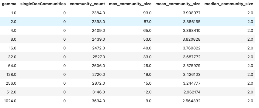
The table shows that increasing gamma reduced the size of the largest community from 93 nodes down to 9 nodes. I thought the smaller communities would have a better chance of capturing nuanced differences between themes.
I selected several themes and took a look at the other themes that were included in their community at various levels of gamma.
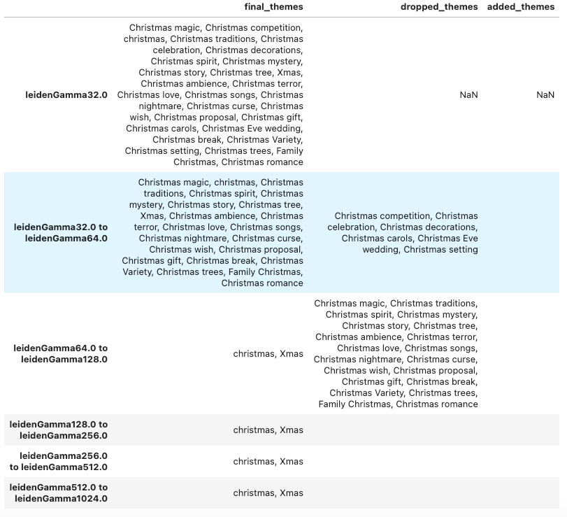
At gamma of 32.0, all of the themes related to Christmas have something to do with the holiday. However, “Christmas terror” and “Christmas miracle” were still together like they were when I tried WCC. When I increased gamma to 128 and above, the other themes dropped out, but “Xmas” and “christmas” remained together.
Based on looking at several different themes at a range of gamma levels, I chose to collect themes in the same Leiden community at a gamma level of 256.0 into the same theme group. For each community, I created a ThemeGroup node. I created IN_GROUP relationships that related the Theme nodes in the community to the ThemeGroup.
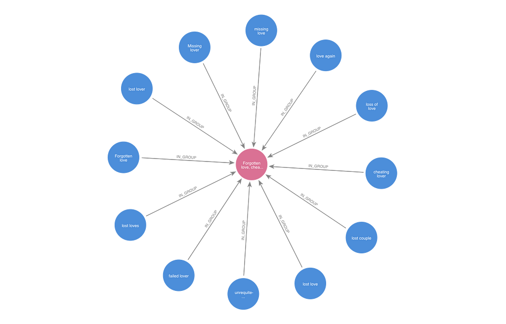
With the theme groups in place, I could begin to query the graph to find movies that shared the same or similar themes. In the example below, two films shared the theme “Opulent neighborhood.” They are also related to a third film that has the theme “opulent home” because both themes are in the same theme group.

Summarize Theme Groups
Once the theme groups were determined, I asked OpenAI’s ChatGPT-3.5-turbo to write a short description of the theme group. The code for this task is in the Summarize theme groups.ipynb notebook. I provided the first sentence of the description following the pattern “These movies address the theme …” Along with the starter sentence, I gave the LLM a sample of up to twenty titles and overviews containing the theme. Here’s the prompt I used.
You are a movie expert.
You will be given a list of information about movies and the first
sentence of a short paragraph that summarizes themes in the movies.
Write one or two additional sentences to complete the paragraph.
Do not repeat the first sentence in your answer.
Use the example movie information to guide your description of the
themes but do not include the titles of any movies in your sentences.
Given a theme group that included “locals vs visitors”, “guest”, “guests”, “visitor”, “visitors” the LLM came up with this summary:
These movies address the themes “locals vs visitors”, “guest”, “guests”, “visitor”, and “visitors.” These movies explore the dynamics between locals and visitors, often highlighting the tension and intrigue that arise when individuals from different backgrounds interact. The narratives delve into the complexities of hospitality, relationships, and the unexpected connections that can form between guests and hosts, visitors and locals. The themes of “locals vs visitors” and “guests” are intricately woven into the storytelling, offering a rich tapestry of human experiences and interactions.
A theme group of “Swindling”, “scam artist”, “scamming”, “swindle” produced this summary:
These movies address the themes “Swindling”, “scam artist”, “scamming”, and “swindle.” These movies delve into the world of deception and manipulation, where characters resort to swindling and scamming to achieve their goals. The narratives explore the consequences of these actions, revealing the complexities of human nature and the blurred lines between right and wrong in the pursuit of personal gain. The characters’ journeys of self-discovery through deceit shed light on the darker aspects of society and the lengths individuals are willing to go to in order to fulfill their desires.
Each summary included all the associated themes in the starter sentence, so no keywords were left out of the summary. The LLM seemed to do a good job of drawing from the movie examples to provide context around the one or two-word themes.
In addition to this long description of the theme group generated by the LLM, I created a short description that followed the pattern “Movies about <concatenated list of themes>.” The short summary for the theme group above was “Movies about Swindling, scam artist, scamming, and swindle”. This allowed me to test whether the extra context provided by the LLM resulted in better retrievals.
I created three vector properties associated with each theme group. I generated embeddings of the short and long summaries using OpenAI’s text-embedding-3-small model. The third embedding was an average of the embeddings of the theme keywords associated with the theme group.
Compare Retrievers Based on Different Vector Indexes
At this point, I had created five vector indexes related to the movie content:
- An index on Movie nodes covering title and overview
- An index on Theme nodes covering the theme words
- An index on ThemeGroup nodes covering the long LLM-generated summary of the theme
- An index on ThemeGroup nodes covering the short summary of the theme “Movies about …”
- An index on ThemeGroup nodes covering the average of the theme vectors from the Theme nodes related to the ThemeGroup
I tested all five indexes with the same set of questions to see which did the best job of retrieving relevant movies. I allowed each index to find up to 50 movies for each question. I focused on recall by counting the number of resulting movies that matched the question for each index. I chose that metric because processes downstream of the retrieval could handle filtering out false positives and ranking the documents. The code for these comparisons is in the Compare retrievers.ipynb notebook.
These were the questions I tested:
- What are some documentaries about painters?
- What are some movies about classical music?
- What are some movies about ice hockey?
- What are some movies about baseball?
- What are some who-done-it movies?
- What are some dark comedies?
- What are some set in Europe in the 1960s?
- What are some movies about pre-Columbian America?
- What are some movies about birds?
- What are some movies about dogs?
Retrieving data from the Neo4j knowledge graph gave me the flexibility to semantically search for vectors similar to my query and then traverse relationships in the graph to find the movies I was looking for.
For the movie index, I retrieved the 50 movies whose vectors most closely matched the query vector. This was the most basic retrieval. Here’s the Cypher query I used.
CALL db.index.vector.queryNodes("movie_text_vectors", 50, $query_vector)
YIELD node, score
RETURN $queryString AS query,
"movie" AS index,
score, node.tmdbId AS tmdbId, node.title AS title, node.overview AS overview,
node{question: $queryString, .title, .overview} AS map
ORDER BY score DESC
For the theme index, I retrieved the 25 theme nodes whose vectors were closest and then used the HAS_THEME relationships in the graph to find all the related movies to those themes. I returned the top 50 movies related to the themes sorted by theme similarity to the query and then movie similarity to the query. I used this Cypher query.
CALL db.index.vector.queryNodes("theme_vectors", 50, $query_vector)
YIELD node, score
MATCH (node)<-[:HAS_THEME]-(m)
RETURN $queryString AS query,
"theme" AS index,
collect(node.description) AS theme,
gds.similarity.cosine(m.embedding, $query_vector) AS score,
m.tmdbId AS tmdbId, m.title AS title, m.overview AS overview,
m{question: $queryString, .title, .overview} AS map
ORDER BY score DESC, gds.similarity.cosine(m.embedding, $query_vector) DESC
LIMIT 50
For the indexes related to theme groups, I found the 25 theme groups that most closely matched the query vector. I used the IN GROUP relationships to find all the themes related to those theme groups. Then, I used the HAS_THEME relationships to find all the movies related to those themes. I returned the top 50 movies sorted by theme group similarity to the query and then movie similarity to the query. Here’s the Cypher query I used to retrieve movies based on the long summary index on the theme group. The queries for short summary and mean indexes were the same except for the index name.
CALL db.index.vector.queryNodes("theme_group_long_summary_vectors",
  25, $query_vector) YIELD node, score
MATCH (node)<-[:IN_GROUP]-()<-[:HAS_THEME]-(m)
RETURN $queryString AS query,
"theme_group_long" AS index,
collect(node.descriptions) AS theme,
gds.similarity.cosine(m.embedding, $query_vector) AS score,
m.tmdbId AS tmdbId, m.title AS title, m.overview AS overview,
m{question: $queryString, .title, .overview} AS map
ORDER BY score DESC,
gds.similarity.cosine(m.embedding, $query_vector) DESC
LIMIT 50
I asked ChatGPT-3.5-turbo to decide whether the movies retrieved were a match for the question. I also judged the movies myself to see if I thought they matched the intent of my question. In some cases, it was a close call. Should a movie about softball count for the baseball question? At what point does a horror movie seem campy enough to count as a dark comedy? I tried to answer consistently, and I made sure that I didn’t know which index had returned the movie when I graded the answers. I found that I agreed with ChatGPT about 74% of the time on whether the movies matched the questions. Overall, I classified more retrieved movies as being relevant to the questions than ChatGPT did.
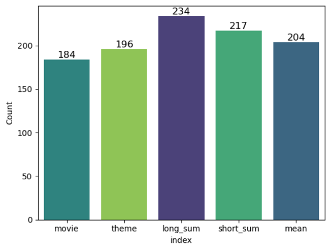
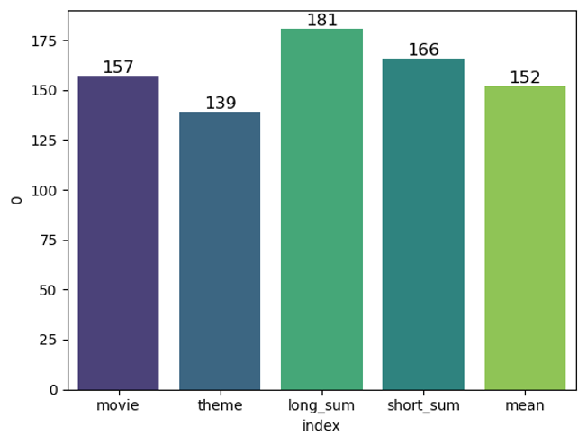
When I summed the total number of movies that I counted as relevant across all questions, the theme group index clearly outperformed the others, finding 27% more relevant movies than the movie index. I could also see that creating ThemeGroup nodes with Graph Data Science gave me better results than using the raw Theme nodes generated by the LLM.
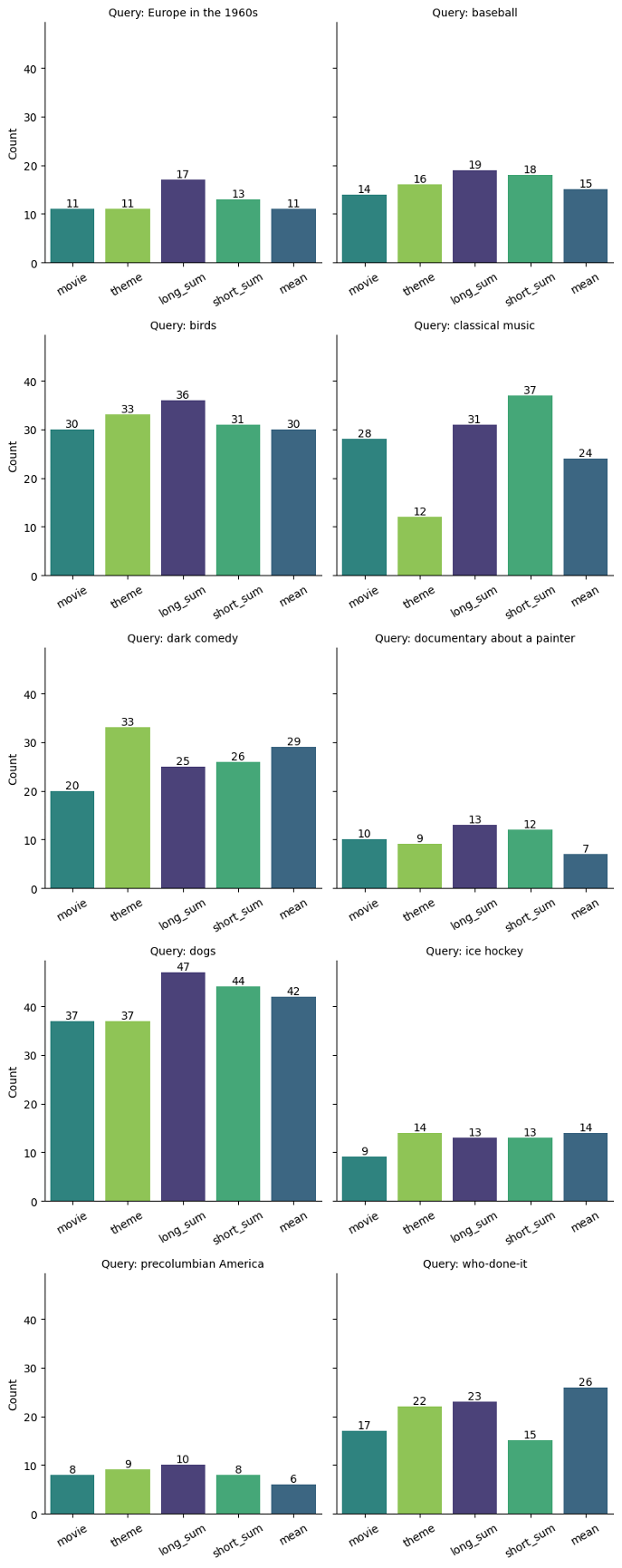
The charts below show a break of the results by the query. While the long summary index was consistently a good performer, and it always outperformed the basic movie index, it wasn’t the top index for every question.
The theme index did exceptionally well at finding dark comedies. It honed in on a theme of “horror comedy” that the long summary index passed over in favor of themes about darkness.
The short summaries index outperformed other indexes on the classical music question. It picked up the theme group, including the word “composer” that other indexes missed.
If we look at the total number of movies that ChatGPT-3.5-turbo thought were relevant, the long summary index still outperformed the others, but it only beat the movie index by 13%. This might be a more realistic expectation for what we would see in a Retrieval Augmented Generation application, where an LLM would analyze the retrieved documents and decide what to rephrase when passing results back to the user.
Conclusion
I saw three key benefits of using Neo4j Graph Data Science for topic modeling in semantic search.
- The long summary theme group index created with Neo4j Graph Data Science provided a larger number of relevant search results than the other indexing strategies.
- Creating the theme groups turned unstructured text into a knowledge graph that could be used for analysis and visualization of the data.
- Performing topic modeling in Neo4j gave me a nice way to stay organized and show my work through the layers of topic extraction, stemming, and topic clustering. Data ingestion and cleaning, algorithmic analysis, and vector-based retrieval all happened in the same graph platform.
Topic Extraction with Neo4j GDS for Better Semantic Search in RAG Applications was originally published in Neo4j Developer Blog on Medium, where people are continuing the conversation by highlighting and responding to this story.
Share Article


Explore
Related Articles


Everything a Developer Needs to Know About the Model Context Protocol (MCP)
25 min read

A Practical Experimentation of GraphRAG and Agentic Architecture With NeoConverse
13 min read
Graphiti: Knowledge Graph Memory for a Post-RAG Agentic World
5 min read